{r setup, include=FALSE} knitr::opts_chunk$set(eval = FALSE) 本文于r format(Sys.Date(), "%Y-%m-%d")更新。 如发现问题或者有建议,欢迎提交 Issue
{r message=FALSE, warning=FALSE, include=FALSE} library(tidyverse)
比较主要参考 @Ng2018SVM,相关PPT详见课程PPT。
Large Margin Classification
@Ng2018SVM [Part 1]主要介绍三方面内容:
- SVM的代数定义,ReLU函数的类似。
- SVM的几何定义,
- SVM代数和几何定义的联系。
SVM的代数定义
SVM的代数定义,是逻辑回归的改进。 我们说理解一个公式了一回事,范化一个公式是另一回事。
Abstract is the price of generation.
这里因此尽可能的举特例快速弄懂。 我们知道逻辑回归, $$z=h_{\theta}(x)=\theta^{T}x$$ $$y=\frac{1}{1+e^{-z}}$$
几个函数的直观理解
{r} tibble(x = c(-10,10)) %>% ggplot(aes(x=x)) + stat_function(fun = function(x){exp(-x)}) + annotate("text", x = 0, y = 10000, parse = TRUE, label = "y == e ^ {-x}") tibble(x = c(-10,10)) %>% ggplot(aes(x=x)) + stat_function(fun = function(x){1/(1+exp(-x))}) + annotate("text", x = 0, y = 0.5, parse = TRUE, label = "y == frac(1, 1 + e ^ {-x})")
我们尽可能的希望,
- 当$y\to1$时,那么$\theta^{T}x\geq0$,且$\theta^{T}x \to + \infty$
- 当$y\to0$时,那么$\theta^{T}x\leq0$,且$\theta^{T}x \to - \infty$
损失函数
上面这是我们的假设,我们要用损失函数实现它。
比如 $$\begin{alignat}{2} \text{Cost} & = -[\overbrace{y\log (h_{\theta}(x))}^{\text{y = 1}}+\overbrace{(1-y)\log(1-h_{\theta}(x))}^{\text{y = 0}}] \ & = -y\log\frac{1}{1+e^{-\theta^Tx}}-(1-y)\log(1-\frac{1}{1+e^{-\theta^Tx}}) \end{alignat}$$
当$y=1$时,
$$\text{Cost}=-\log\frac{1}{1+e^{-\theta^Tx}}=\log(1+e^{-\theta^Tx})$$
{r} tibble(x = c(-10,10)) %>% ggplot(aes(x=x)) + stat_function(fun = function(x){log(1+exp(-x))}) + annotate("text", x = 0, y = 5, parse = TRUE, label = "y == log(1 + e ^ {-x})")
当$y=0$时,
$$\text{Cost}=-\log(1-\frac{1}{1+e^{-\theta^Tx}})=\log(1+e^{\theta^Tx})$$
{r} tibble(x = c(-10,10)) %>% ggplot(aes(x=x)) + stat_function(fun = function(x){log(1+exp(x))}) + annotate("text", x = 0, y = 5, parse = TRUE, label = "y == log(1 + e ^ {x})")
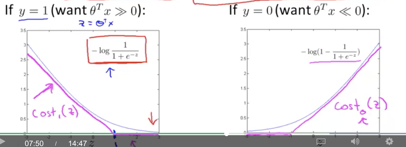
- 当$y=1$时,只要$\theta^Tx\geq0$,那么$Cost=0$。
- 当$y=0$时,只要$\theta^Tx\leq0$,那么$Cost=0$。
这个就是ReLu函数。
注意这里我们可以用更严格的条件,
- 当$y=1$时,只要$\theta^Tx\geq1$,那么$Cost=0$。
- 当$y=0$时,只要$\theta^Tx\leq-1$,那么$Cost=0$。
这里就把逻辑回归,中间这种0两边突变的情况考虑了,因此对cutoff不那么灵敏了,因此效果好、稳定。
$C$参数调整正则化强度。
SVM的几何定义
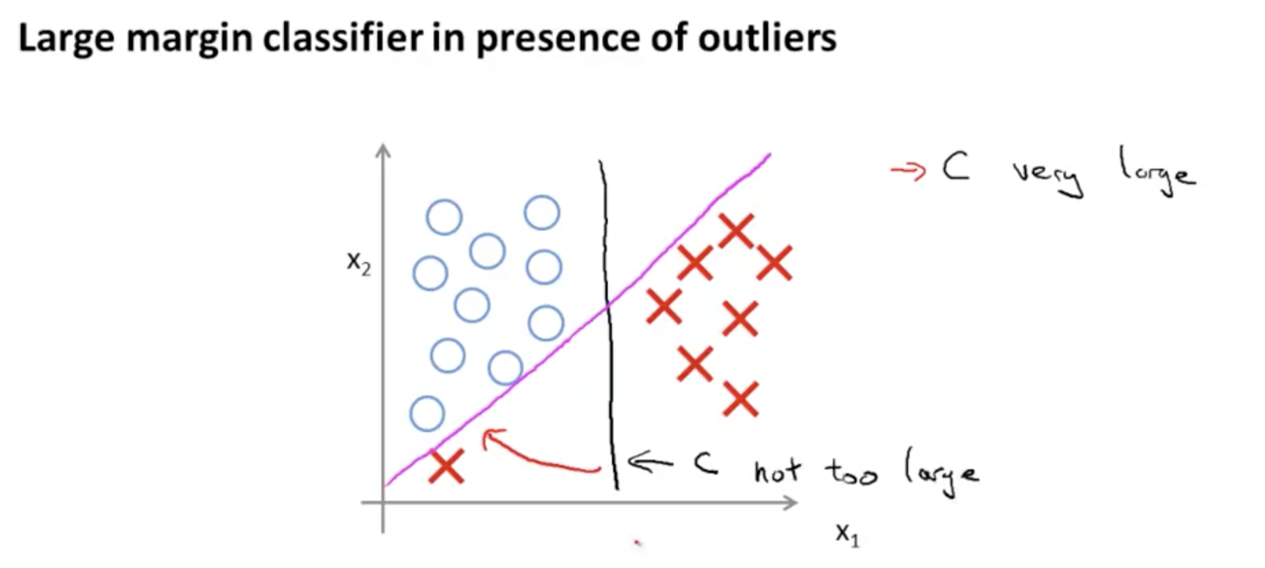
显然C很大的时候,分割线旋转,导致将outlier进行了切分。 旋转的原因见 @ref(relation)。
SVM代数和几何定义的联系
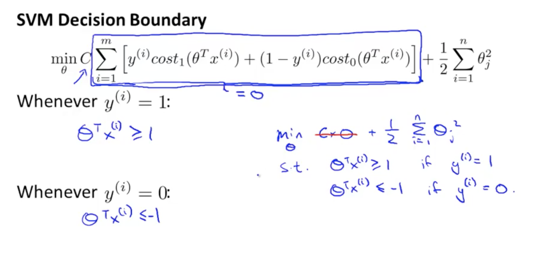
这是代数定义里面我们要完成的任务,
- 当$y=1$时,只要$\theta^Tx\geq1$,那么$Cost=0$。
- 当$y=0$时,只要$\theta^Tx\leq-1$,那么$Cost=0$。
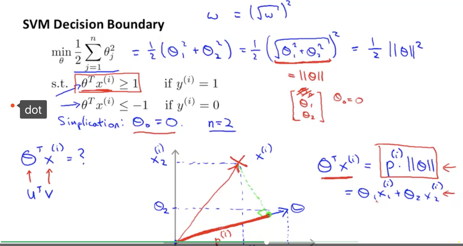
- 也就是说,$|\theta^Tx|\geq1$ $\to$ 点积$x_i|\theta|\geq1$ $\to$ 因此$x_i$要足够大。 $\to$ $x$在$\theta$上的投影要足够大。 。
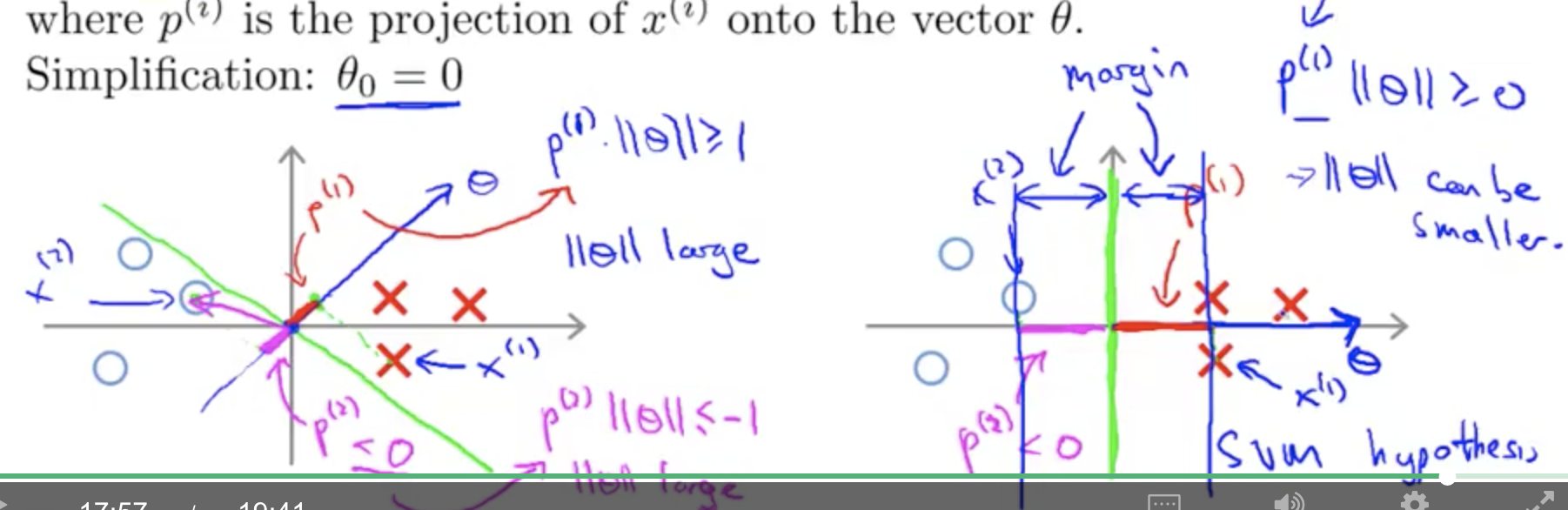
因此我们会发现, $x$在$\theta$上的投影要足够大。 等价于 $x$在$\theta$的法向量距离足够大。 因此这就是代数定义和图形定义的联系。
kernel 函数
损失函数
@ref(linear)的损失函数是线性模型,采用了类似于Relu函数的操作 这里介绍一个基于正态分布完成了的cost函数,这种函数在SNE也有涉及。 可以处理类别被包围的情况。
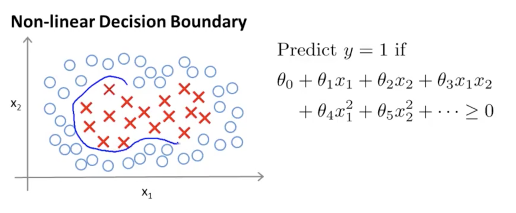
我们知道多项式,例如$x_1^2 +x_2^2$可以表达圆,通过$x_1^2 +x_2^2\sim0$的关系,完成圆内和圆外的关系, 但是除了多项式,还有正态分布这种方式。
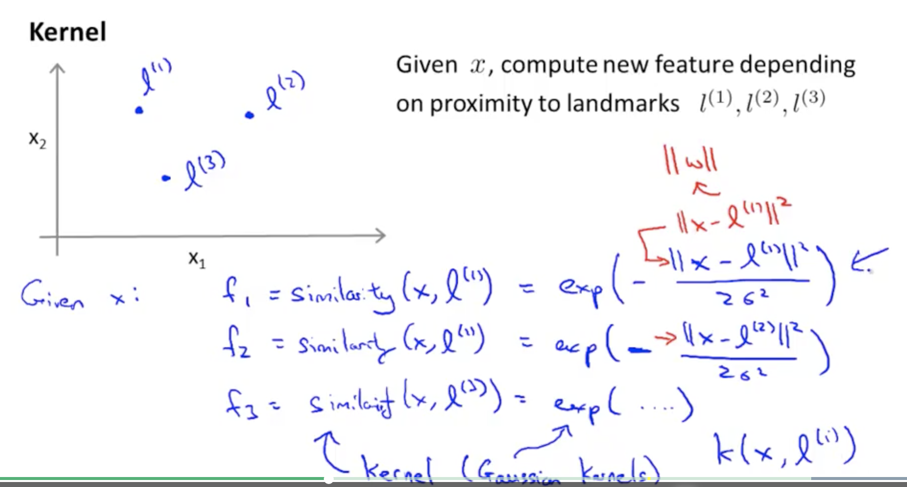
如图我们在图中选择这些点,通过将该点作为频率分布图的中心,做高斯分布, 那么周围$\forall x$离该点$l^{(1)}$的距离判断,两点的相似程度,similarity。 那么,
$$f_1 = \text{similarity}(x,l^{(1)})=\exp(-\frac{||x-l^{(1)}||^2}{2\sigma^2}) \in [0,1]$$
因此可得到,
Gaussian Kernel函数,
$$\begin{alignat}{2} f_1 & = \text{similarity}(x,l^{(1)})=\exp(-\frac{||x-l^{(1)}||^2}{2\sigma^2}) \in [0,1]\ f_2 & = \text{similarity}(x,l^{(2)})=\exp(-\frac{||x-l^{(2)}||^2}{2\sigma^2}) \in [0,1]\ \cdots \ f_m & = \text{similarity}(x,l^{(m)})=\exp(-\frac{||x-l^{(m)}||^2}{2\sigma^2}) \in [0,1]\ \end{alignat}$$
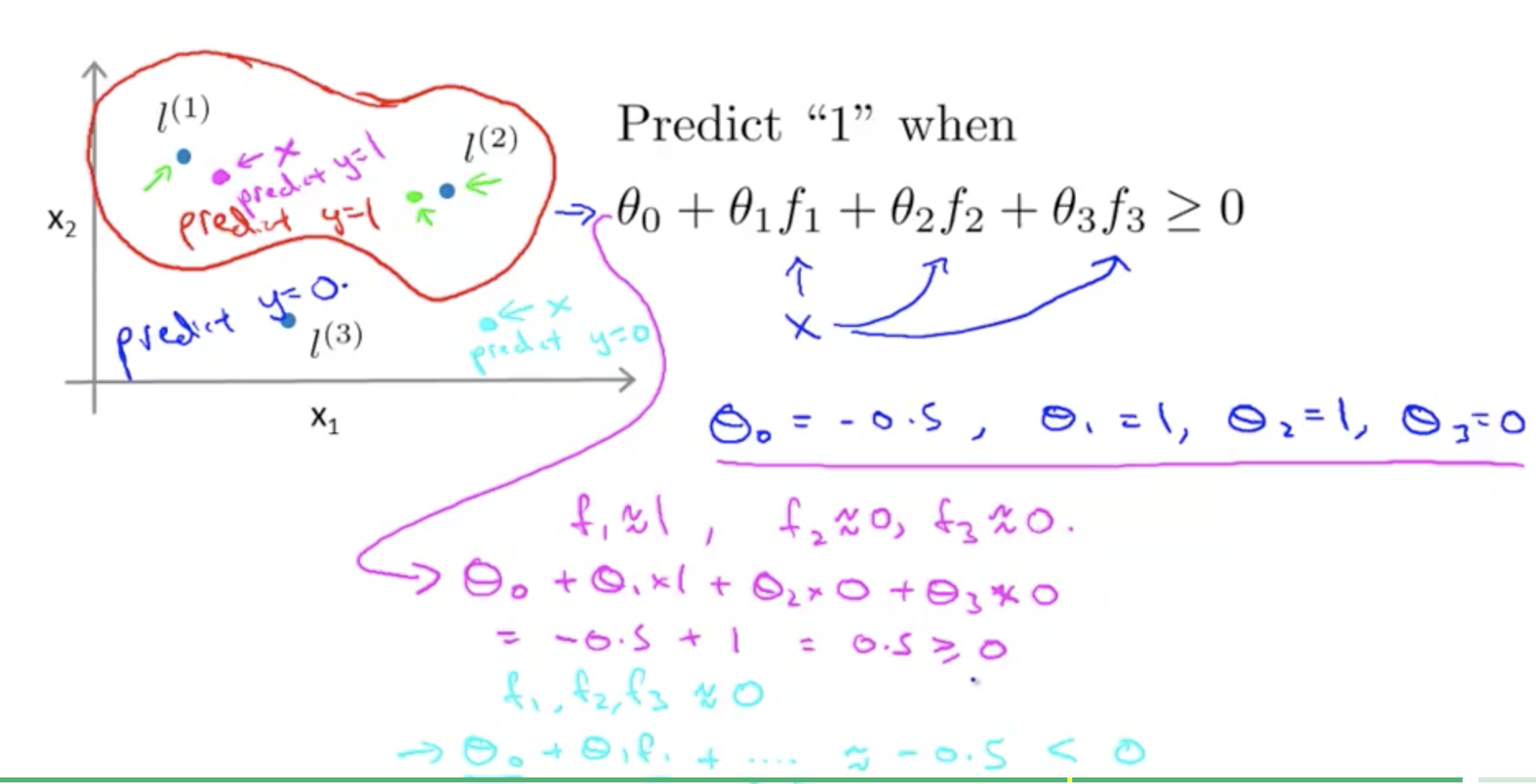
$$\begin{alignat}{2} \hat y=1\gets & \theta^Tx\geq 1\ & \theta_0 + \theta_1x_1 + \theta_2x_2 + …\ \end{alignat}$$
现在换成,
$$\begin{alignat}{2} \hat y=1\gets & \theta^Tf\geq 1\ & \theta_0f_1 + \theta_1f_1 + \theta_2f_2 + …\ \end{alignat}$$
假设$f_0 = 1$
- 我们认为$y=1$在圆外,因此$\theta^Tf\geq >0$明显在圆外,
- 我们认为$y=0$在圆内,因此$\theta^Tf\leq <0$明显在圆内。
这个时候我们把这个关系整理到cost函数中,就是
$$\min_{\theta}C\sum_{i=1}^my^{(i)}cost_1(\theta^Tf^{(i)})+(1-y^{(i)})cost_0(\theta^Tf^{(i)})+\frac{1}{2}\sum_{j=1}^m\theta_j^2$$
后面的思路就是应用到SVM了。 因此现在SVM我们掌握了两种方法,一种是ReLu函数,一种是Gaussian Kernel函数。
实际操作
SVM线性核函数的推荐
- Use linear kernel when number of features is larger than number of observations (@ref(morefeature)).
- Use gaussian kernel when number of observations is larger than number of features.
- If number of observations is larger than 50,000 speed could be an issue when using gaussian kernel; hence, one might want to use linear kernel. [@Temlyakov2013]
总计一句话就是,都先尝试线性模型,在线性模型效果不好的情况下,再考虑使用非线性模型。
- polynomial -> 把直线变弯
- radial -> 变球
变量多用线性模型
当特征向量的数量远大于样本数量,样本之间会比较稀疏, 因此更高维度的空间,样本之间会比较稀疏,更容易线性可分。 因此用线性模型。 但是,如果数据密集,就不容易线性可分了。
- 因此当样本量小于特征向量时,特征已经足够,更多体现了线性关系(甚至可能存在共线性关系),这时就没有必要使用Gaussian Kernel函数了。
- 因此当样本量大于特征向量时,
- 特征不足够,
- 且样本不是特别大而影响速度,
- 需要体现非线性关系,这时就需要使用Gaussian Kernel函数了。见CSDN博客,第6和12点