{r setup, include=FALSE} knitr::opts_chunk$set(eval = FALSE)
<iframe frameborder="no" border="0" marginwidth="0" marginheight="0" width="330" height="86" src="//music.163.com/outchain/player?type=2&id=520706973&auto=1&height=66">
</iframe>
Inference for Numerical Data
- 4 hours
- 15 Videos
- 50 Exercises
- 232 Participants 学的人更少,说明这个东西反向来看,日后必然是重点,注重统计方法的实现,是sense,是data exploring的想法。
Mine Cetinkaya-Rundel 这个老师我很喜欢。
什么是bootstrap
Bootstraping scheme
- Take a bootstrap sample - a random sample taken with replacement from the original sample, of the same size as the original sample.
- Calculate the bootstrap statistic - a statistic such as mean, median, proportion, etc. computed on the bootstrap samples.
- Repeat steps (1) and (2) many times to create a bootstrap distribution - a distribution of bootstrap statistics.
也就是说,
$$bootstrap = same \space size + replace$$
library(infer)

___ %>%                               # start with data frame
  specify(response = ___) %>%         # specify the variable of interest
  generate(reps = ___, type = "bootstrap") %>%  # generate bootstrap samples
  calculate(stat = "___")             # calculate bootstrap statistic
这个包真好!!!
什么是t分布?
首先理解什么是t分布? 假设$X_1,\cdots,X_n$n个变量,都服从正态分布$\mathcal N \sim (\mu,\sigma)$。 因此我们定义 $\bar X = \frac{1}{n}\sum_{i=1}^nX_i$ 但是我们会发现这里样本标准差要小一些,为什么? $s^2 = \frac{1}{n-1}\sum_{i=1}^n(\bar X - X_i)^2$ 为什么要除以$n-1$, 因为我们做了一次平均,类似于减小波动的手法, 因此$\bar X$的波动理论上就是要小于$\forall X_i$的,这是直觉的理解。
为什么t分布是n-1的自由度?
以上我们发现,t分布就是找一波相同正态分布的变量作为样本,然后求样本的分布,计算均值和方差, 因此我们经过了一步均值处理,这就是关键,这就是为什么自由度减小了。
举个例子,你有$a,b,c,d$,每个变量都很自由,想选什么就选什么,没有约束条件。 这时,你非要假设你知道了均值,比如5,那么这个时候 $a+b+c+d=20$,然后就减少了1个自由度。 为什么?因为现在的预算是4个自由度,
- 假设你给了a,a可以随机选择,比如$a=5$,那么$5+b+c+d=20$。
- 假设你给了b,b可以随机选择,比如$b=2$,那么$5+2+c+d=20$。
- 假设你给了c,c可以随机选择,比如$c=0$,那么$5+2+0+d=20$。
这个时候,d根本不自由,只能等于8了,这个时候就发现,当我们做了均值假设的时候,我们就少了一个自由度的预算,变成三个了,也就是$df=4-1$。
Generate bootstrap distribution for median | R
因此我们发现t分布是很多正态分布均值化而来的,我们做个模拟。
```{r eval=F} # ,cache =T manhattan <- read_csv( “https://assets.datacamp.com/production/course_5103/datasets/manhattan.csv ) # Generate bootstrap distribution of medians rent_ci_med <- manhattan %>% # Specify the variable of interest specify(response = rent) %>%
# Generate 15000 bootstrap samples generate(reps = 15000, type =“bootstrap”) %>% # Calculate the median of each bootstrap sample calculate(stat = “median”)
View the structure of rent_ci_med
str(rent_ci_med)
Plot a histogram of rent_ci_med
ggplot(rent_ci_med, aes(stat)) + geom_histogram(binwidth = 50)
当我们说一个样本满足t分布时候,
我们就在说,这个样本的样本均值,
是将每个样本看成了一个变量,
看这个样本均值的波动了。
假设
`manhattan`满足t分布,
那么里面每一个样本都是一个$X_i$变量了。
我们求中位数,这个中位数算出来是一个值,但是实际上是一个分布的观察值。
因为我们拿到的样本实际上是变量的观测值。
这个时候我们要看这个中位数的分布,我们可以使用bootstrap。
因为这些样本都是同一个正态分布的,
因此我们可以假设bootstrap后,等到的其他样本(变量)也是类似的,
可以求出其他样本的中位数,那么这些中位数虽然是观测值,但是它们就组成了一个近似的分布,
因此我们得到了分布。

因此为什么我们要bootstrap15000次求中位数。

* [Review percentile and standard error methods | R](https://campus.datacamp.com/courses/inference-for-numerical-data/bootstrapping-for-estimating-a-parameter?ex=3)

percentile methods

bootstrap 后,用distribution来算置信区间。

standard error methods

更精确,

$$sample \space stats \pm t_{df=n-1}\times se_{boot}$$

### [Calculate bootstrap interval using both methods | R](https://campus.datacamp.com/courses/inference-for-numerical-data/bootstrapping-for-estimating-a-parameter?ex=4)

既然我们已经拿到了median这个指标的t分布,我们就开始计算他的平均数和标准差了,
注意平均数和标准差是针对这个median指标的。
因此任何的样本statistic都可以有t分布,可以算出一个均值和标准差,
而且可以通过bootstrap做出这个statistic的分布。

`dplyr::pull()`就是把一个$1\times1$table变成数字。

```
# Percentile method
rent_ci_med %>%
  summarize(l = quantile(stat, 0.025),
            u = quantile(stat, 0.975))

# Standard error method

# Calculate observed median
rent_med_obs <- manhattan %>%
  # Calculate observed median rent
  summarize(median(rent)) %>%
  # Extract numerical value
  pull()

# Determine critical value
t_star <- qt(0.975,  df = nrow(manhattan)-1)

# Construct interval
rent_ci_med %>%
  summarize(boot_se = sd(rent_ci_med$stat)) %>%
  summarize(l = rent_med_obs - t_star * boot_se,
            u = rent_med_obs + t_star * boot_se)
用原样本的中位数,这个中位数就是个观察值 用bootstrap的标准差,因为这个标准差bootstrap后的、中位数的标准差,是一个被平均过指标,被$\frac{1}{\sqrt{n}}$。
Great job! The standard error method is more appropriate here.
了解下infer包
在generate函数中, reps表示
the number of resamples to generate, 是__resamples__的简称。
bootstrap和 permute的区别是 permute是随机置换顺序 。
Permuation是对已有的样本进行重新排序,打乱之前对照组和实验组的差异。 而Bootstrap是从样本中重复抽样。 [@Yu2012]
we shift the bootstrap distribution to be centered at the null value.
p-value = The proportion of simulations that yield a sample statistic at least as favorable to the alternative hypothesis as the observed sample statistic.
当假设了$\mathcal H_0$,bootstrap的分布的形状不变,平移到$\mathcal H_0$处,这个时候$\sigma$不变,但是$\mu$变了,仅此而已。
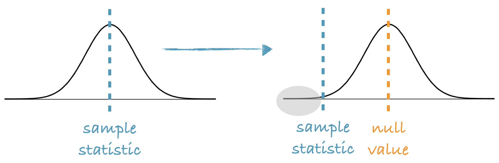
所以是用sample stats的均值去做检验。
null: the null hypothesis. Options include “independence” and “point
```{r} # Generate 15000 bootstrap samples centered at null set.seed(123) rent_med_ht <- manhattan %>% specify(response = rent) %>% hypothesize(null = “point”, med = 2500) %>% #对rent值没有影响,在bootstrap环节有。 generate(reps = 15000, type = “bootstrap”) %>% #产生replicate就是编号 calculate(stat = “median”)
Calculate observed median
rent_med_obs <- manhattan %>% summarize(median(rent)) %>% pull()
Calculate p-value
rent_med_ht %>% filter(stat > rent_med_obs) %>% summarize(n() / nrow(rent_med_ht))
在这个地方,`stat`已经代表了population的值,
而`rent_med_obs`就是个样本值在检验。
`summarise((n()/1500)*2)`要是双侧,`*2`。
这里怎么理解,就是找小的阴影部分面积$\times 2$,
简单来说就是
+ `stat > rent_med_obs`,`rent_med_obs`大,超过均值线,所以,这样写。
+ `stat < rent_med_obs`,`rent_med_obs`小,未超过均值线,所以,这样写。
* [t-distribution | R](https://campus.datacamp.com/courses/inference-for-numerical-data/introducing-the-t-distribution?ex=1)
t分布与正态分布的区别之一依然是去估计,$\bar x$,但是$\sigma$是未知的,需要知道df。
因为df之小,因此t分布尾巴比正太分布大,具体理解为图。
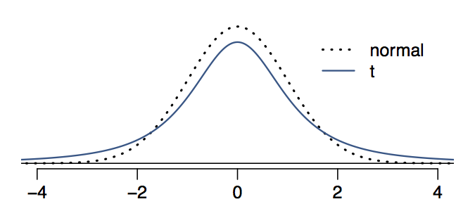
因此可以理解为t分布中,大多数点更可能落在$\bar x \pm 2\sigma$之外。
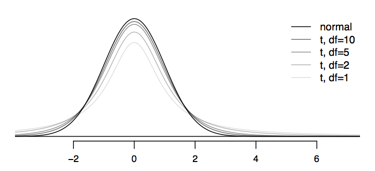
如图,随着$df=(n-1)$增加,t分布更加趋近于正态分布。
注意这个地方只是$\sigma$不知道,但是样本依然是
__随机的__,
__分布形状__
还是知道的(t分布)。
* [Probabilities under the t-distribution | R](https://campus.datacamp.com/courses/inference-for-numerical-data/introducing-the-t-distribution?ex=3)
对于t分布,已知
cutoff `q`
自由度 `df`后,
可以知道$P(x < q)$,
使用`pt(q = T, df)`实现。
```
# P(T < 3) for df = 10
# 位于分布右边
(x <- pt(q = 3, df = 10))
# P(T > 3) for df = 10
(y <- 1-x)
# P(T > 3) for df = 100
(z <- 1-pt(q = 3, df = 100))
# Comparison
y == z
y > z
y < z
(x <- pt(q = 3, df = 10))位于分布右边,由于长尾巴,因此是偏小的 $\to$ (y <- 1-x)偏大。
-
pt(q, df): q,df$\to$p prob. -
qt(p, df): p,df$\to$q cutoff
这里 q指的是quantiles, p指的是probabilities。
```{r} # 95th percentile for df = 10 (x <- qt(p=0.95, df = 10))
upper bound of middle 95th percent for df = 10
(y <- qt(p=0.975,df=10))
upper bound of middle 95th percent for df = 100
(z <- qt(p=0.975,df=100))
Comparison
y == z y > z y < z
```
library(tidyverse)
expand.grid(
  df = seq(1,100,1),
  p  = seq(0.8,0.999,0.001)
) %>%
  mutate(q = qt(p = p, df = df)) %>%
  ggplot(aes(x = df, y = log(q))) +
  geom_point(alpha = 0.25)
如图,相同概率下,df$\uparrow$ $\to$ q$\downarrow$,因为尾巴越来越小。
我们要求样本间相互独立,但是这本身很难,有一个弱条件,实际中可以使用。
-
随机抽样,
-
如果
replace = FALSE,那么 $n < 10%$ of N,不能太多。 -
如果skew严重,n要更大些,靠谱。
<!-- -->
# Subset for employed respondents
acs12_emp <- acs12 %>%
  filter(employment == "employed")

# Construct 95% CI for avg time_to_work
t.test(acs12_emp$time_to_work, conf.level = 0.95)

> # Subset for employed respondents
> acs12_emp <- acs12 %>%
    filter(employment == "employed")
>
> # Construct 95% CI for avg time_to_work
> t.test(acs12_emp$time_to_work, conf.level = 0.95)

    One Sample t-test

data:  acs12_emp$time_to_work
t = 32.635, df = 782, p-value < 2.2e-16
alternative hypothesis: true mean is not equal to 0
95 percent confidence interval:
 24.43369 27.56120
sample estimates:
mean of x
 25.99745
这里的t.test得到的区间,感觉和我们的bootstrap得到的结果类似啊。
是不是估计的总体均值的区间。 这里这样理解, 我们这里有两个$\mu$,
- 一个是我们假设的总体$\mu$,
- 一个是我们计算的的样本$\bar x$。
我们可以bootstrap我们的样本,得到一个分布。
- 这个分布 + $\mu$ $\to$ $\bar x$的显著水平,p值多少。
- 这个分布 + $\bar x$ $\to$ $\mu$的置信区间,如果置信区间钟不包含$mu$,那么我们假设的$\mu$不成立。
这里的思想就是$\mu$和$\bar x$通过t分布,互相佐证。
很有sense的一个例子。
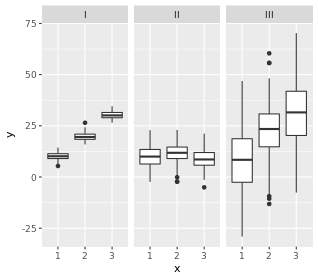
200 observations were randomly sampled from the High School and Beyond survey.The same students took a reading and writing test. At a first glance, how are the distributions of reading and writing scores similar? How are they different?
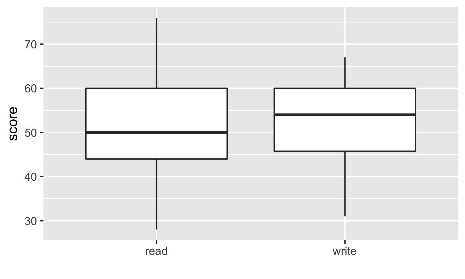
我们要假设的就是, 是否这两种成绩之间没有线性关系,比如reading高,writing就一定高。反面就是,是否两者更能独立?
对箱形图的理解, 两个分布还是有点不一样的。 在read图中,median位置,靠近25%,因此说明有right tail。 在read图中,25-75%更宽,因此说明方差更大。
paired data的t检验就是,找$\Delta = x_1-x_2$来做t检验就好了。
t.test(hsb2$diff, conf.level = 0.95)
    One Sample t-test

data:  hsb2$diff
t = -0.86731, df = 199, p-value = 0.3868
alternative hypothesis: true mean is not equal to 0
95 percent confidence interval:
 -1.7841424  0.6941424
sample estimates:
mean of x
   -0.545
We are 95% confident that the average reading score is 1.78 points lower to 0.69 points higher than the average writing score.
0在中间,所以independent的假设是拒绝的。
-
confidence level 95%
-
significance level 5%
Do the data provide convincing evidence of a difference between the average reading and writing scores of students? Use a 5% significance level.
- 从conf. interval 的角度,这是看一个stats的波动范围。
- 从signif. interval 的角度,这是看一个$\mathcal H_0$的是否成立。
这里使用 t.test(hsb2$diff, null = 0, alternative = "two.sided"), 中间使用的是null = 0, alternative = "two.sided", 标准的testing语言, 而非之前我们算confidence level的语言 t.test(hsb2$diff, conf.level = 0.95)。
注意p值大的情况,确实0值在confidence level其中。
t.test(hsb2$diff, null = 0, alternative = "two.sided")
    One Sample t-test

data:  hsb2$diff
t = -0.86731, df = 199, p-value = 0.3868
alternative hypothesis: true mean is not equal to 0
95 percent confidence interval:
 -1.7841424  0.6941424
sample estimates:
mean of x
   -0.545
Suppose instead of the mean, we want to estimate the median difference in prices of the same textbook at the UCLA bookstore and on Amazon. You can’t do this using a t-test, as the Central Limit Theorem only talks about means, not medians. You’ll use an
inferpipeline to estimate the median.
这也算是bootstrap的一个理由。
# Calculate 15000 bootstrap means
textdiff_med_ci <- textbooks %>%
  specify(response = diff) %>%
  generate(reps = 15000, "bootstrap") %>%
  calculate(stat = "median")

# Calculate the 95% CI via percentile method
textdiff_med_ci %>%
  summarise(l = quantile(stat, 0.025),
            u = quantile(stat, 0.975))

# A tibble: 1 x 2
      l     u
  <dbl> <dbl>
1  5.04 11.73
试验结果就是书店平均状态下更贵,在亚马逊上买。 这就是实验目的,实验设计的很简单,但是很实用。
这里sense最重要,内容很简单,因此要留心。
Conduct the hypothesis test.
Write the values of change on 18 index cards.
(1) Shuffle the cards and randomly split them into two equal sized decks: treatment and control 1.
(2) Calculate and record the test statistic: difference in average change between treatment and control.
Repeat (1) and (2) many times to generate the sampling distribution.
Calculate p-value as the percentage of simulations where the test statistic is at least as extreme as the observed difference in sample means.
因此permute是随机的,因此样本均值的差应该为0。 如果说permute一下,就没有差异了,那么就说明之前的差异是巧合。这里permute,切换了位置,好比因为这次冲击,产生的一种必然现象,不受到random assignment影响。
{r} library(openintro) data(stem.cell)
library(infer)

diff_ht_mean <- stem.cell %>%
  specify(__) %>%                    # y ~ x
  hypothesize(null = __) %>%         # "independence" or "point
  generate(reps = _N_, type = __) %>%# "bootstrap", "permute", or "simulate
  calculate(stat = "diff in means")  # type of statistic to calculate
y这里是响应变量reponse variable 2, x这里是解释变量explantory variable,就是treatment group。 这里选择"independent"是因为,我们假设y ~ treatment是独立的。
因此最后我们计算的p value就是
$$P( (\bar x_{(treat,obs)}-\bar x_{(ctrl,obs)}) < (\bar x_{(treat,sim)}-\bar x_{(ctrl,sim)}) )$$
这里的$sim$代表了总体方程。
这里treat和ctrl组分别有before和after,因此我终于明白了为什么有点复杂。 这里before和after,重要的是他们的差值。
```{r} library(tidyverse) # Calculate difference between before and after stem.cell <- stem.cell %>% mutate(change = after-before)
Calculate observed difference in means
diff_mean <- stem.cell %>% # Group by treatment group group_by(trmt) %>%
# Calculate mean change for each group summarise(mean_change = mean(change)) %>% # Extract pull() %>% # Calculate difference diff()
diff_mean
* [Evaluating the effectiveness of stem cell treatment (cont.) | R](https://campus.datacamp.com/courses/inference-for-numerical-data/inference-for-difference-in-two-parameters?ex=3)

```
# Generate 1000 differences in means via randomization
library(infer)
diff_ht_mean <- stem.cell %>%
  # y ~ x
  specify(change ~ trmt) %>%
  # Null = no difference between means
  hypothesize(null = "independence") %>%
  # Shuffle labels 1000 times
  generate(reps = 1000, type = "permute") %>%
  # Calculate test statistic
  calculate(stat = "diff in means", order = c("esc", "ctrl"))

# Calculate p-value
diff_ht_mean %>%
  # Identify simulated test statistics at least as extreme as observed
  filter(stat > diff_mean) %>%
  # Calculate p-value
  summarize(p_val = n() / 1000)
calculate出现的问题,需要加入order3。
We want to evaluate whether there is a difference between weights of babies born to smoker and non-smoker mothers.
$$weights \sim oke$$
stat 4在这里选择"diff in means"。
# Remove subjects with missing habit
ncbirths_complete_habit <- ncbirths %>%
  filter(!is.na(habit))

# Calculate observed difference in means
diff_mean <- ncbirths_complete_habit %>%
  # Group by habit group
  group_by(habit) %>%
  # Calculate mean weight for each group
  summarize(mean_weight = mean(weight)) %>%
  # Extract
  pull() %>%
  # Calculate difference
  diff()

# Generate 1000 differences in means via randomization
diff_ht_mean <- ncbirths_complete_habit %>%
  # y ~ x
  specify(weight ~ habit) %>%
  # Null = no difference between means
  hypothesize(null = "independence") %>%
  # Shuffle labels 1000 times
  generate(reps = 1000, type = "permute") %>%
  # Calculate test statistic
  calculate(stat = "diff in means")

# Calculate p-value
diff_ht_mean %>%
  # Identify simulated test statistics at least as extreme as observed
  filter(diff_mean > stat) %>%
  # Calculate p-value
  summarize(p_val = (n()/1000)* 2)

> mean(diff_ht_mean$stat)
[1] -0.0028943

> diff_mean
[1] -0.3155425
很显然,diff_mean$<$mean(diff_ht_mean$stat),位于左侧,因此算 $2\timesP$(diff_mean$<$mean(diff_ht_mean$stat))。
我们知道confidence interval w/ 95% 就是 significant level 5%,两者互换,刚才计算了significant level的p值,现在可以计算confidence interval了。
- 针对一个参数(或者两个参数的change)的时候,我们使用bootstrap,
- 针对两个参数的时候,我们使用permute。
Bootstrap CI for a difference
- Take a bootstrap sample of each sample - a random sample taken with replacement from each of the original samples, of the same size as each of the original samples.
- Calculate the bootstrap statistic - a statistic such as difference in means, medians, proportion, etc. computed based on the bootstrap samples.
- Repeat steps (1) and (2) many times to create a bootstrap distribution - a distribution of bootstrap statistics.
- Calculate the interval using the percentile or the standard error method 5.
<!-- -->
# Generate 1500 bootstrap difference in means
diff_mean_ci <- ncbirths_complete_habit %>%
  specify(weight ~ habit) %>%
  generate(reps = 1500, type = "bootstrap") %>%
  calculate(stat = "diff in means")

# Calculate the 95% CI via percentile method
diff_mean_ci %>%
  summarize(l = quantile(stat, 0.025),
            u = quantile(stat, 0.975))

# A tibble: 1 x 2
           l           u
       <dbl>       <dbl>
1 -0.5856007 -0.05373011
为什么这里使用type = "bootstrap"? 因为这里最后给到一个区间,在smoke和nonsmoke之间换位置,算confidence interval还是不妥吧。 因此两遍各自bootstrap比较科学。 这个地方需要总结下的。 理解起来也比较直观。6
<!-- -->
# Remove subjects with missing habit and weeks
ncbirths_complete_habit_weeks <- ncbirths %>%
  filter(!is.na(habit),!is.na(weeks))

# Generate 1500 bootstrap difference in medians
diff_med_ci <- ncbirths_complete_habit_weeks %>%
  specify(weeks ~ habit) %>%
  generate(reps = 1500, type = "bootstrap") %>%
  calculate(stat = "diff in medians")

# Calculate the 92% CI via percentile method
diff_med_ci %>%
  summarise(l = quantile(stat, 0.04),
            u = quantile(stat, 0.96))

# A tibble: 1 x 2
      l     u
  <dbl> <dbl>
1    -1     0
使用公式,算出三个指标。
{r echo=FALSE, message=FALSE, warning=FALSE} tibble::tribble( ~citizen, ~x_bar, ~s, ~n, "no", 21.19, 34.5, 58L, "yes", 18.52, 24.73, 901L ) %>% knitr::kable()
<!-- -->
> t.test(hrly_pay ~ citizen, data = acs12_complete_hrlypay_citizen)

    Welch Two Sample t-test

data:  hrly_pay by citizen
t = 0.58058, df = 60.827, p-value = 0.5637
alternative hypothesis: true difference in means is not equal to 0
95 percent confidence interval:
 -6.53483 11.88170
sample estimates:
 mean in group no mean in group yes
         21.19494          18.52151
开始多个means比较。
{r} download.file("https://assets.datacamp.com/production/course_5103/datasets/gss_wordsum_class.csv", "gss.csv") gss <- read_csv("gss.csv") ggplot(gss, mapping = aes(x = wordsum)) + geom_histogram(binwidth = 1) + facet_grid(class ~ .)
facet_grid(class ~ .)和facet_grid(~ class)是完全不一样的,如果更加care $x$坐标,就用前者。 这个不需要ggridge也可以完成。
但是这个图显然需要facet_grid(~ class)了,因为更加care$y$轴。
<!-- 开始讲F检验了。 -->
<!-- 这里定义了between group 和within group 两种vars。 -->
通过anova检验,理解$R^2$、$R_{adj.}^2$、$F$值
{r} tibble::tribble( ~term, ~df, ~sumsq, ~meansq, ~statistic, ~p.value, "class", 3L, 236.5644, 78.85481, 21.73467, 0L, "Residuals", 791L, 2869.8003, 3.628066, NA, NA ) %>% knitr::kable()
<!-- 这是anova检验的结果,怎么解读呢? -->
首先class相当于一个分类变量,类似于回归中的$x$, Residuals是未解释部分,类似于回归中的$\hat \mu$。 df=3是因为这里有四类,去掉一个对照组,失去了三个自由度。 791是剩余的自由度(n-1-k)。
sumsq表示波动,236.5644是解释部分,2869.8003是未解释部分,因此,
$$R^2 = \frac{236.5644}{236.5644+2869.8003}$$
其中meansq = sumsq/df。 这里的
$$F = \frac{78.854810}{3.628066}$$
根据这个特性,
$$R_{adj.}^2 = 1- \frac{\frac{2869.8003}{791}}{\frac{236.5644+2869.8003}{791+3}}$$
感觉和F值很类似啊,都是求单位自由度的波动。 因为都是考虑了波动和自由度的两个因素。
{r} aov_wordsum_class <- aov(wordsum ~ class, data = gss) library(broom) tidy(aov_wordsum_class)
aov(formula, data = NULL。
这里主要讲了anova的适用条件。
Conditions for ANOVA
Independence:
- within groups: sampled observations must be independent 7
- between groups: the groups must be independent of each other (non-paired)
Approximate normality8: distribution of the response variable should be nearly normal within each group
Equal variance: groups should have roughly equal variability 9
{r} library(broom) pairwise.t.test(x = gss$wordsum, g = gss$class, p.adjust = "none") %>% tidy()
就可以比较两两之间的t检验了。
但是这里的t值的阈值有所改变。 因为假设我们使用5%,如果每个两两之间都还是用5%,那么总体上看,我们的容忍度必然超过了5%,不科学。因此我们用$\frac{5%}{K}$,这个$K$代表了我们一共需要进行多少次比较,即:
$$C_k^2=\frac{k(k-1)}{2}$$
这也是Bonferroni correction。
-
注意这个地方, (1) 为什么要这么做,就是和python的统计思维那篇一样,认为两者是相同的,treat = ctrl,然后进行permute,最后拿到新的$\mu = x_{treat}-X_{ctrl}$,模拟一个distribution, 最后用真实的$\mu = x_{treat}-X_{ctrl}$来比较。 这个permute的统计思维要多训练几次,才搞得清楚。 ↩︎
-
证明之前的是
y ~ 1,因为只有一个parameter要检验。 ↩︎ -
因此加入
order = c("first", "second")。
↩︎Error in calculate(., stat = "diff in means") : Statistic is a difference, specify the `order`` in which to subtract. Check `?calculate` for details. -
a string giving the type of the statistic to calculate. Current options include “mean”, “median”, “sd”, “prop”, “diff in means”, “diff in medians”, “diff in props”, “Chisq”, “F”, and “slope”. ↩︎
-
这里就是计算原来样本的stat $\pm t_{原样本n, \alpha/2}\times se_{boot}$ ↩︎
-
计算confidence interval的时候肯定是boostrap的。 但是进行检验的时候,可是使用permute这种换位置更加严格的方法。 ↩︎
-
随机抽样且占比总体的10%。 ↩︎
-
特别是样本小,但是可以通过visualization来观察,比如histogram图。 ↩︎
-
可以通过visualization来观察。
{r} gss %>% group_by(class) %>% summarise(sd(wordsum))↩︎