{r setup, include=FALSE} knitr::opts_chunk$set(eval = FALSE) 本文于r format(Sys.Date(), "%Y-%m-%d")更新。 如发现问题或者有建议,欢迎提交 Issue
intro
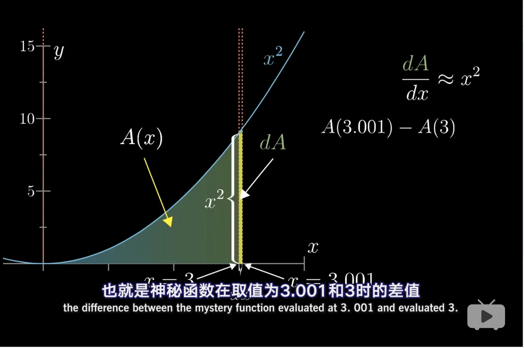
分析方法,用面积来看待这个问题,迎刃而解。 [@3Blue1Browncalculus01]
$$\frac{dA}{dx} = x^2$$
$$dA = x^2 dx$$
因此产生了微分的概念。
导数的悖论
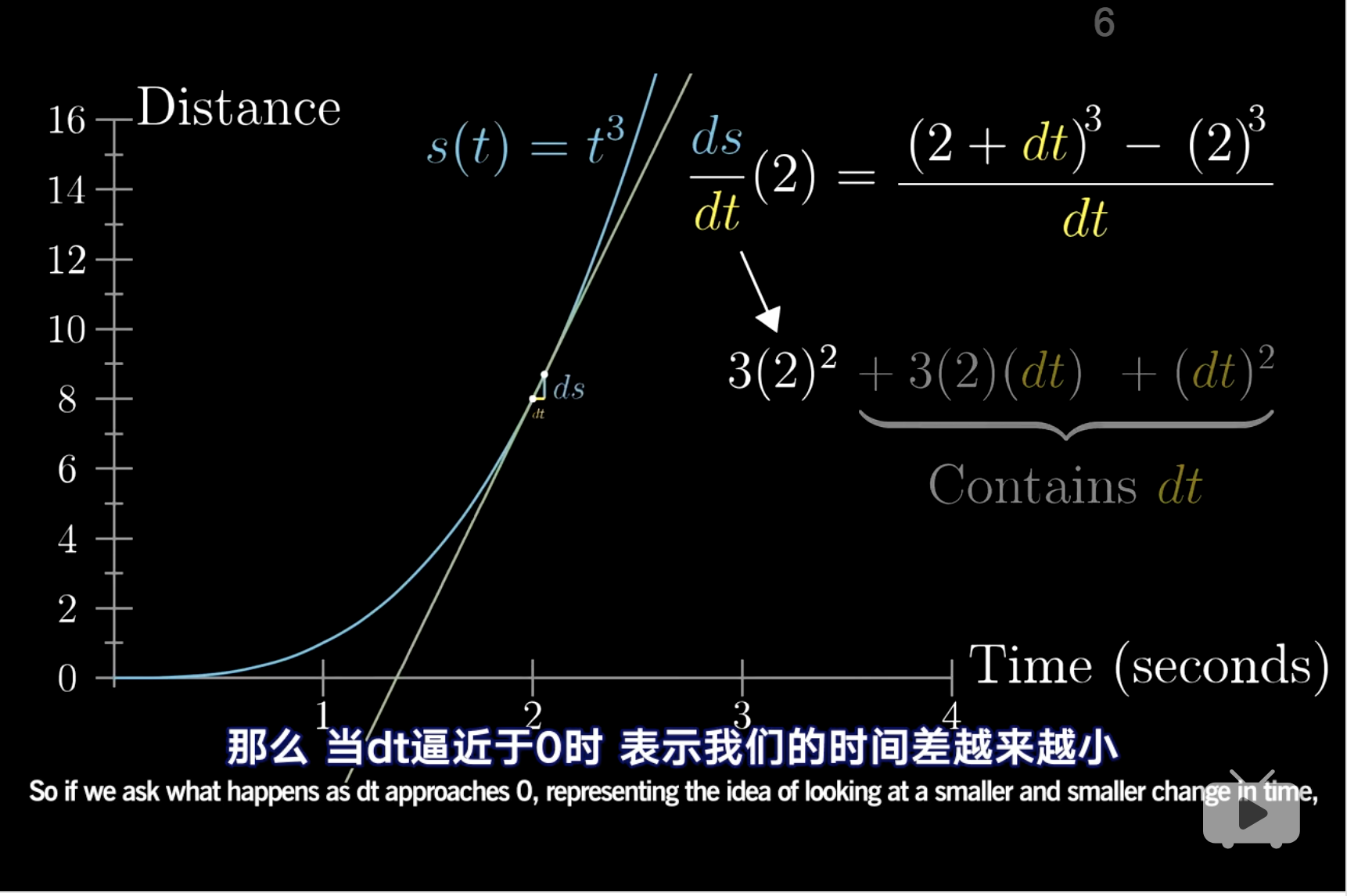
这是强推的方式,但是非常有直觉理解求导的意义,单纯的背公式,已经让人忘记了最初的想法。
另外导数不是瞬时变化率,而是最接近$x = x_0$时的最近似的瞬时变化率的估计值,因为这里是一个平均的概念。 [@3Blue1Browncalculus01]
几何法理解
Power Rule
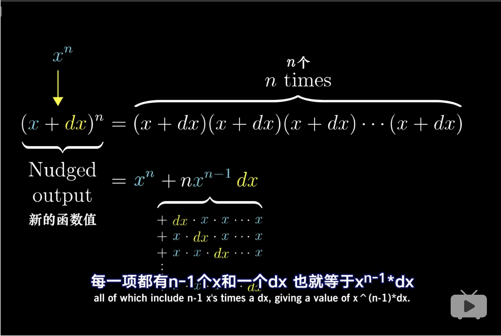
Power Rule 最直观的证明方法。
这里也可以解释
$$(x \cdot y)’ = x’ \cdot y + x \cdot y’ + x’ \cdot y’$$
画一个长方形理解。
inverse proportional function
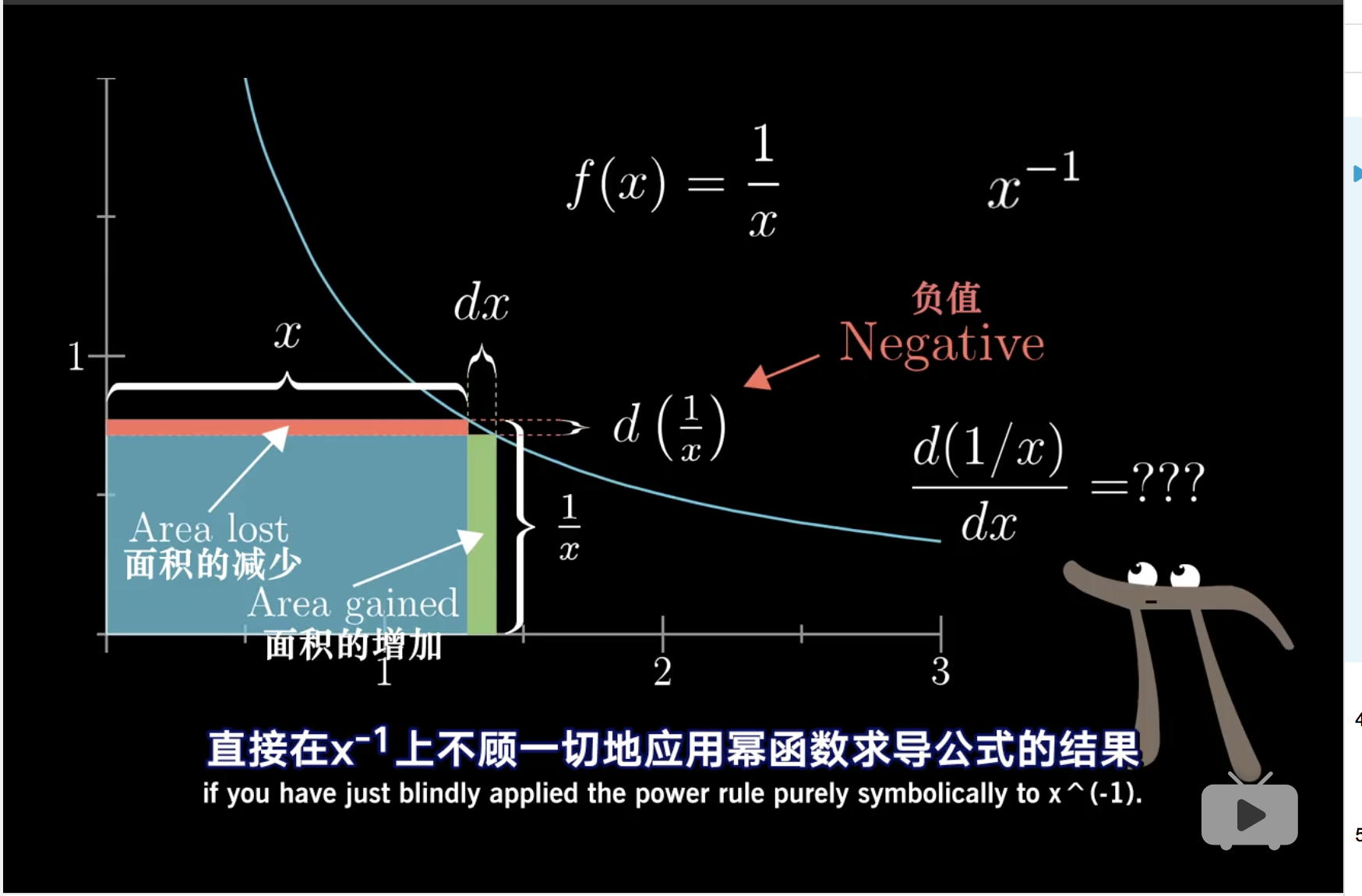
因此,
$$\frac{d}{dx}f(x) = \frac{d}{dx}(\frac{1}{x})$$
因为
$$d(\frac{1}{x}) <0$$
所以
$$\frac{d}{dx}f(x) < 0$$
$$\Delta = x \cdot d(\frac{1}{x}) - dx \cdot \frac{1}{x} \xrightarrow{S=1} 0$$
因为面积恒为1
$$d(\frac{1}{x}) = - \frac{1}{x^2}$$
sqrt function
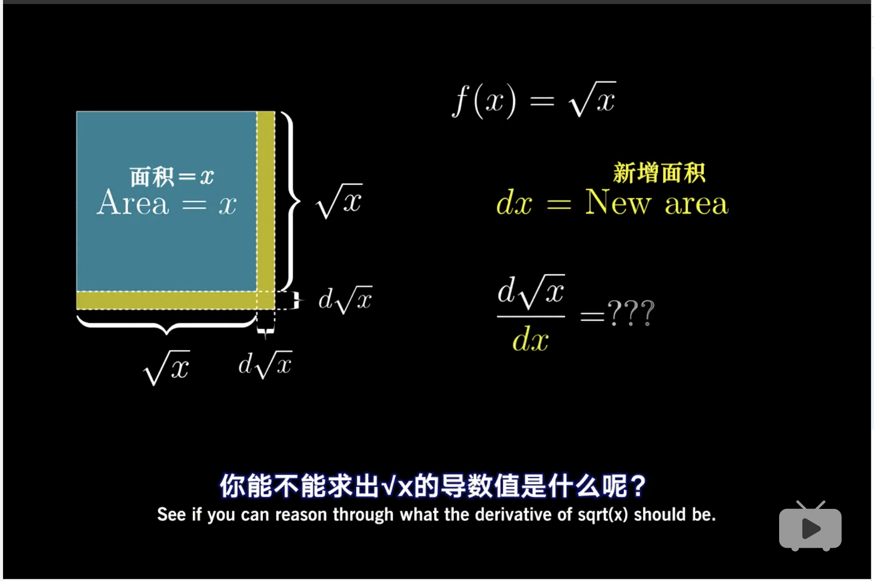
$\Box$没有work out
sine function
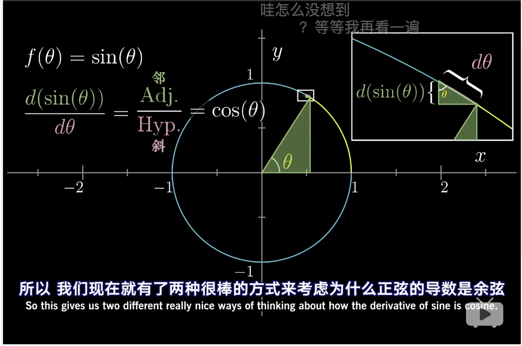
在切点上,满足切线和法线垂直的关系,得两个相似三角形。
因此
$$\frac{d(\sin (\theta))}{d \theta} = \frac{\cos \theta}{r}$$
其中$r = 1$
同理,
$$\frac{d(\cos (\theta))}{d \theta} = - \frac{\sin \theta}{r}$$
Chain Rule
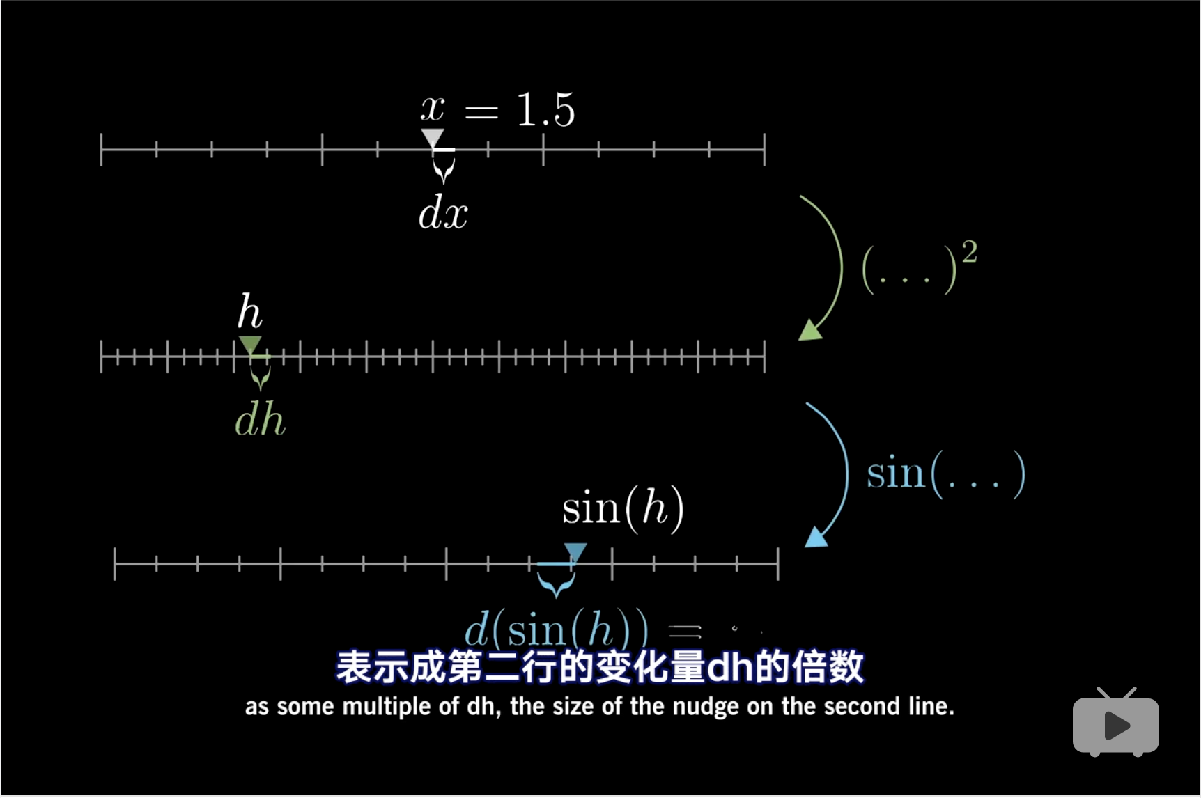
这是Chain Rule 比较直观的理解了,因为需要计算两个以上的导数,因此 @ref(geometricmethod) 就不适用了,而是要采用类似于 @ref(fixedpoint) 的方法。
指数函数求导
这里有两个要点:
- 理解$e$是怎么来的
- 理解$\ln2, \ln3$怎么求出来?为什么要求?
指数函数求导最直观的一个例子。
$$\begin{alignat}{2} M(t) &= 2^t \ \frac{d}{dt}M(t) & \xrightarrow{dt = 1} \frac{2^{t+1}-2^t}{t+1-t} = 2^t \end{alignat}$$
$\Delta$是其本身,也就是翻倍的意思。
进而思考
$$\frac{2^{t+dt}-2^t}{t+dt-t} = 2^t\cdot\frac{2^{dt}-1}{dt}$$
$$\begin{cases}
\frac{2^{0.01}-1}{0.01} = r (2^0.01 - 1)/0.01 \
\frac{2^{0.01}-1}{0.01} = r (2^0.001 - 1)/0.001 \
\frac{2^{0.01}-1}{0.01} = r (2^0.0001 - 1)/0.0001 \
\frac{2^{0.01}-1}{0.01} = r (2^0.00001 - 1)/0.00001 \
\end{cases}$$
我们会发现当$dt \to 0$时, $\frac{2^{dt}-1}{dt}$会收敛于一个点。
进而思考
$$\frac{4^{t+dt}-4^t}{t+dt-t} = 4^t\cdot\frac{4^{dt}-1}{dt}$$
$$\begin{cases}
\frac{4^{0.01}-1}{0.01} = r (4^0.01 - 1)/0.01 \
\frac{4^{0.01}-1}{0.01} = r (4^0.001 - 1)/0.001 \
\frac{4^{0.01}-1}{0.01} = r (4^0.0001 - 1)/0.0001 \
\frac{4^{0.01}-1}{0.01} = r (4^0.00001 - 1)/0.00001 \
\end{cases}$$
我们会发现当$dt \to 0$时, $\frac{4^{dt}-1}{dt}$会收敛于一个点。
那么这个点可否为1?
$$\begin{cases}
\frac{2.7^{dt}-1}{0.00001} = 1 \to r (2.7^0.00001 - 1)/0.00001 \
\frac{2.71^{dt}-1}{0.00001} = 1 \to r (2.71^0.00001 - 1)/0.00001 \
\frac{2.718^{dt}-1}{0.00001} = 1 \to r (2.718^0.00001 - 1)/0.00001 \
\frac{2.7182^{dt}-1}{0.00001} = 1 \to r (2.7182^0.00001 - 1)/0.00001 \
\frac{2.71828^{dt}-1}{0.00001} = 1 \to r (2.71828^0.00001 - 1)/0.00001 \
\end{cases}$$
这就是自然对数产生的意义。
同理,0.69和1.38满足2被关系,2和4也是。
因此猜想,
$$\frac{n^{dt}-1}{dt} \sim n$$
这里使用chain rule, 现在任何数可以用$e^c$表示, 那么,
$$\begin{alignat}{2} 2^t &= e^{\ln (2) \cdot t} \ \frac{d}{dt}2^t &= \frac{d}{dt}e^{\ln (2) \cdot t} = e^{\ln (2) \cdot t} \cdot \ln 2 = 2^t \cdot \ln 2\ \end{alignat}$$
同理,
$$\begin{cases} \frac{d}{dt}2^t & = 2^t\cdot\frac{2^{dt}-1}{dt} &= 2^t \cdot \ln 2 \ \frac{d}{dt}4^t & = 2^t\cdot\frac{4^{dt}-1}{dt} &= 4^t \cdot \ln 4 \ \end{cases}\to \begin{cases} \frac{2^{dt}-1}{dt} &= \ln 2 \ \frac{4^{dt}-1}{dt} &= \ln 4 \ \end{cases} \to \frac{\frac{2^{dt}-1}{dt}}{\frac{4^{dt}-1}{dt}} = \frac{0.69}{1.38} = \frac{2}{4}$$
因此这才是$\ln 2, \ln 4$被求出来的方法和意义。
隐函数求导
implicit differentiation
几何的表达
隐函数求导,几何的表达是,一个点在平面的移动,由$dx$和$dy$来表达。
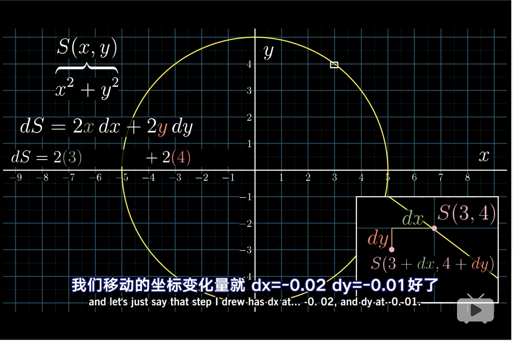
$dS$的变化可以用$dx$和$dy$来表达,进而引出
$$dS = 2x \cdot dx + 2y \cdot dy$$
使得$dS$不变,约束在一个圆上,得到导数$\frac{dy}{dx}$。
对数求导的证明
$$\begin{alignat}{2} \frac{dy}{dx} & = \frac{d}{dx}(\ln x) \ y &= \ln x \ e^y &= x \ e^y \cdot dy &= dx \ \frac{dy}{dx} &= \frac{1}{e^y} \ &= \frac{1}{x} \ \end{alignat}$$
积分和斜率
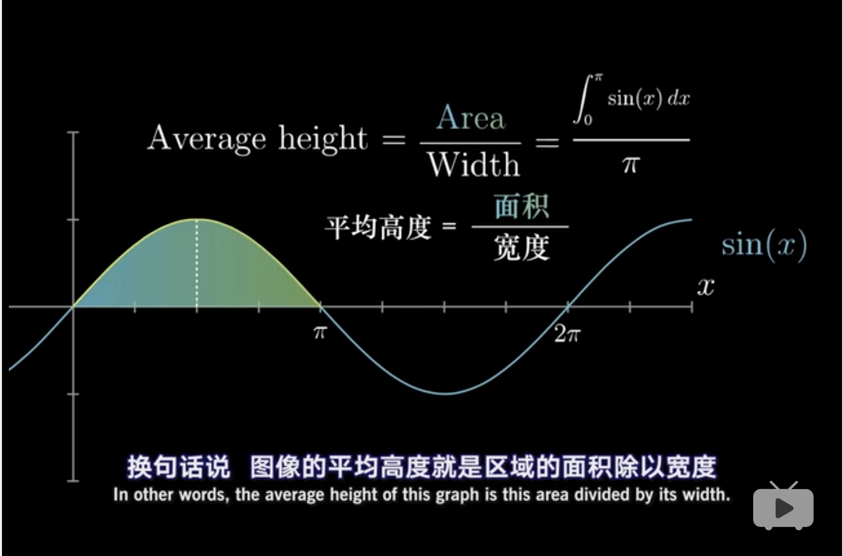
这就是期望的定义。
泰勒级数的理解
泰勒级数的理解,是多项式的求和,因为是多项式,所以易于求导积分。 且泰勒级数在极限条件下,可以对一些非易于求导积分的函数进行拟合。 因此从近似的角度,泰勒级数可以通过代替这些函数,从而完成易于求导积分的作用。
以$$\cos(x) \approx 1-\frac{x^2}{2}$$为例。
假设$$\cos(x)|x = 0$$可以用$$P(x) = c_0+c_1x+c_2x^2$$描述。 至少满足的条件是,在$x =0$时的,常值、一阶导数、二阶导数,两个函数要相似。 即,$$\cos(0)=c_0,\cos(0)’=c_1,\cos(0)’’=c_2$$ 因此, $$\begin{alignat}{2} \cos(x)\xrightarrow{x=0}1& = P(0) = c_0 \ 1 & = c_0 \end{alignat}$$
$$\begin{alignat}{2} \frac{d(\cos)}{d x}(0)=-\sin(0) & =\frac{dP}{dx}(0)=c_1 + 2c_2x \ 0 & = c_1 + 2c_2x = c_1 + 2 \times 0 \ 0 & = c_1 \end{alignat}$$
$$\begin{alignat}{2} \frac{d^2(\cos)}{d x^2}(0)=\cos(0)=-1 & = \frac{d^2(cos)}{dx^2} = 2c_2 \ -1 & = 2c_2 \ -\frac{1}{2} = c_2 \ \end{alignat}$$
所以$c_0,c_1,c_2$都求得了,满足近似的条件。
实际上,$$cos(0.1) \approx1-\frac{1}{2}(0.1)^2 = 0.995$$而, $$cos(0.1)=0.9950042$$
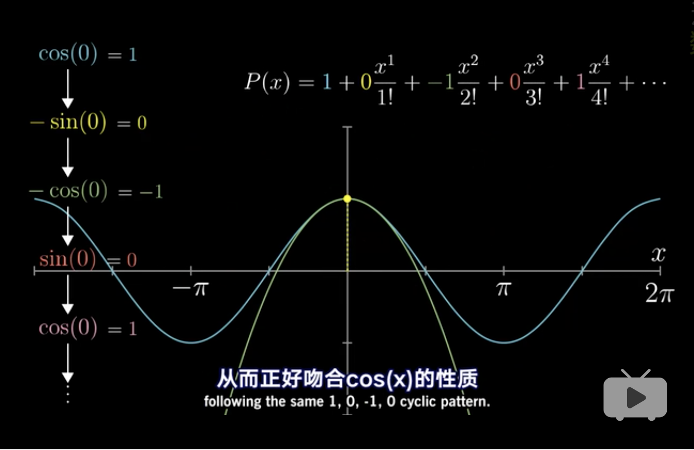
而且我们发现每次多项式求导$$(x^n)’=nx^{n-1}$$ 且$$\frac{d^n(cos)}{dx^n}(0)=n!c_n$$ 所以,$$c_n=\frac{f^{(n)}(0)}{n!}$$
这就还原了泰勒公式了。
$$P(x) = 1 + 0\frac{x^1}{1!} + -1\frac{x^2}{2!} + …$$
其他
不动点和导数
并参考 @3Blue1Browncalculus 的视频讲解而总结。
一种理解导数的方法
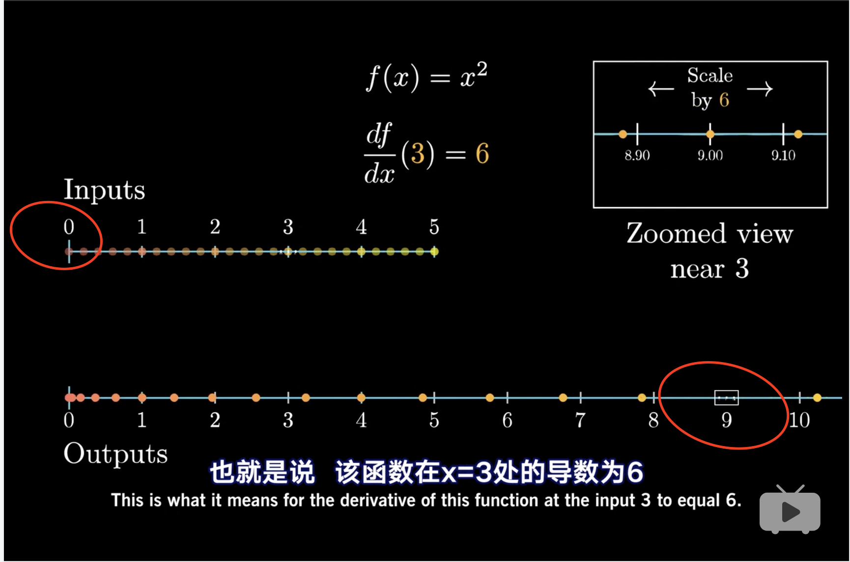
第一轴为x,第二轴为y。 当求在x=3时的导数时,展示y轴上的点是y=9,但是有一个白色小框表示一段波动的距离,这个距离是x轴波动小框的6倍长度,这就是导数的另外一种理解方法。

当求在x=0.1时的导数时,展示y轴上的点是y=0.01,即x和y都是趋近于0的。 但是显然从上面的一个例子的理解上,x的白色小框是大于y的白色小框。
$$导数 = \frac{y轴白色小框}{x轴白色小框} < 1$$
因此说明导数绝对值小于1。
如果我们构建一个不动点公式,
$$x = f(x) = x^2$$
那么这样一直循环下去, x和y都会趋近于0,白色小框越来越窄,最后为0,即"不动"1。
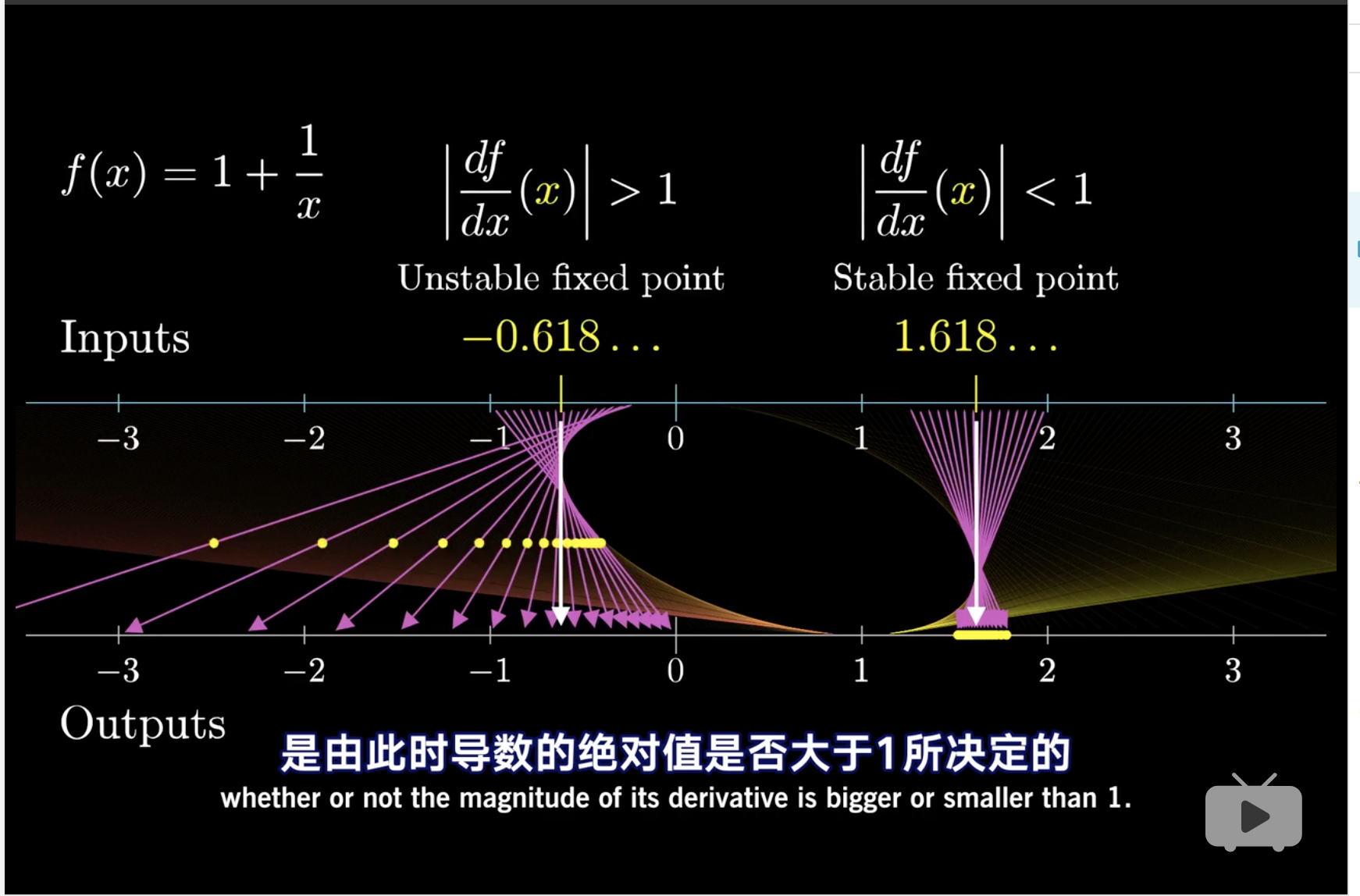
不动点
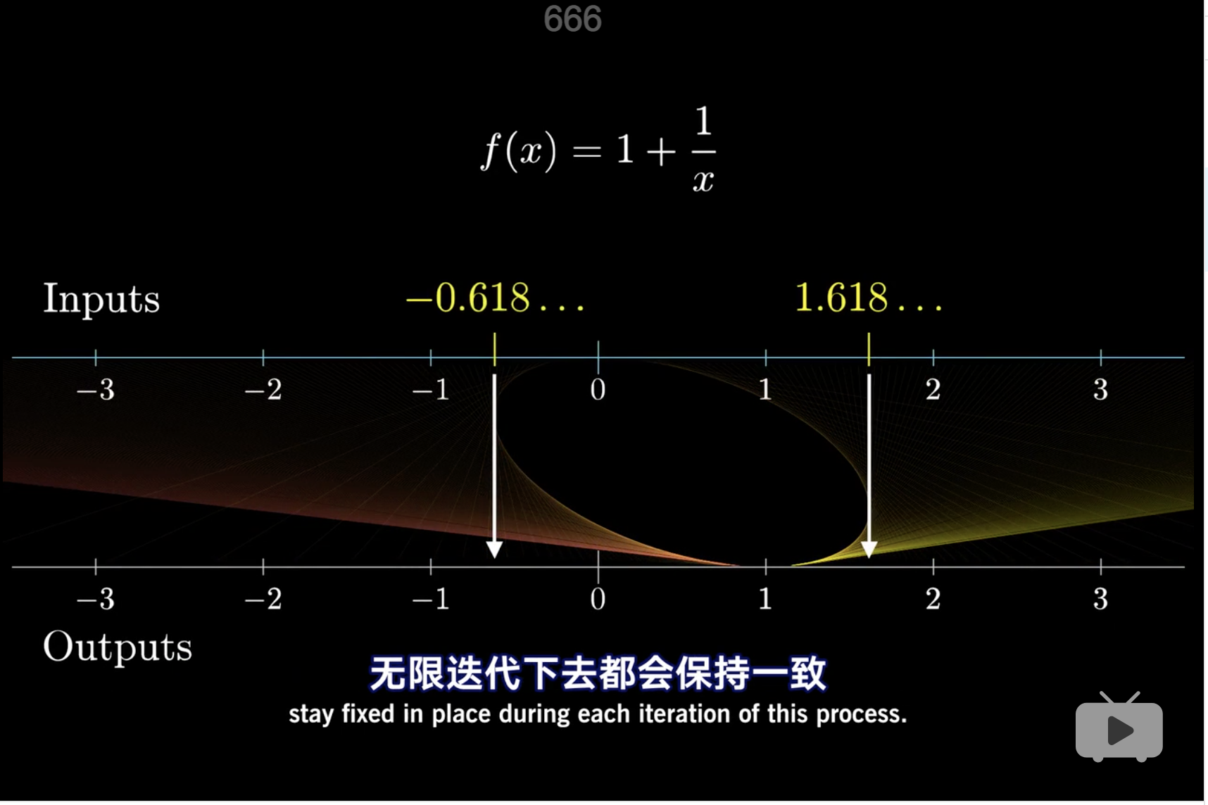
按照以上理解导数的例子,以下这个方程中,x的全集映射在y上,是围绕着y=1的2。

这里的映射关系类似于宇哥椭圆的原因是这原来是由一个圆平移导致3。
这里产生两个不动点
- x = -.618
- $\phi$ = 1.618 4
当x = 1.618附近的一个点,比如x = 2进行迭代时, 白色小框会逐渐缩小,直到消失, 因此这种白色小框缩小的趋势,可以理解为导数一开始就就是绝对值小于1,然后逐渐趋近于不动点。 并且最后的导数趋近于
$$f’\to f’|x = \text{fixed point}$$
{r} library(glue) x <- 2 x = 1 + 1/x;glue("new x value is {round(x,4)} and locally the difference is {round(-1/x^2,4)}") x = 1 + 1/x;glue("new x value is {round(x,4)} and locally the difference is {round(-1/x^2,4)}") x = 1 + 1/x;glue("new x value is {round(x,4)} and locally the difference is {round(-1/x^2,4)}") x = 1 + 1/x;glue("new x value is {round(x,4)} and locally the difference is {round(-1/x^2,4)}") x = 1 + 1/x;glue("new x value is {round(x,4)} and locally the difference is {round(-1/x^2,4)}") x = 1 + 1/x;glue("new x value is {round(x,4)} and locally the difference is {round(-1/x^2,4)}") x = 1 + 1/x;glue("new x value is {round(x,4)} and locally the difference is {round(-1/x^2,4)}") x = 1 + 1/x;glue("new x value is {round(x,4)} and locally the difference is {round(-1/x^2,4)}") x = 1 + 1/x;glue("new x value is {round(x,4)} and locally the difference is {round(-1/x^2,4)}") x = 1 + 1/x;glue("new x value is {round(x,4)} and locally the difference is {round(-1/x^2,4)}") x = 1 + 1/x;glue("new x value is {round(x,4)} and locally the difference is {round(-1/x^2,4)}") x = 1 + 1/x;glue("new x value is {round(x,4)} and locally the difference is {round(-1/x^2,4)}")
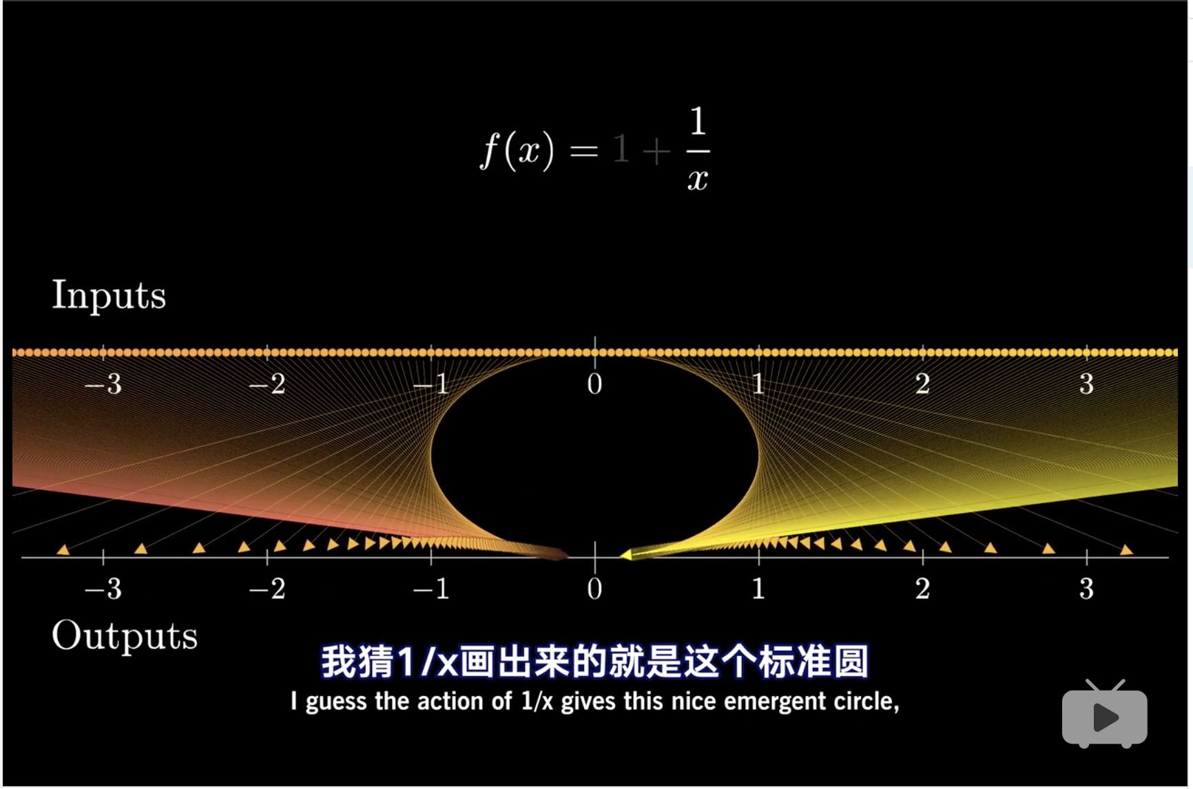 $$f(x) = \frac{1}{x}$$ 向函数 $$f(x) = 1+ \frac{1}{x}$$ 向右平移一个单位得到。