{r setup, include=FALSE} knitr::opts_chunk$set(eval = FALSE) 下载需要的数据
内容多,因此通过修订,方便记忆。 利用结构图,理解各个函数method之间的逻辑。 没有全是md代码和相关的 diagrammR 代码。
新增
- 目录
第一章
```{r echo=FALSE, message=FALSE, warning=FALSE} library(DiagrammeR) grViz( digraph dot {
graph [layout = dot]
node [shape = egg, style = filled, color = darkgreen, fontsize = 12, fontname = Helvetica, fontcolor = white, # label = ‘’]
a [label = ‘read_*’] b [label = ‘pd.DataFrame()’] c [label = ‘.index’] d [label = ‘.columns’] e [label = ‘.values’] f [label = ‘.index.values’] g [label = ‘.columns.values’] h [label = ’np.array’]
edge [ color = darkgreen, fontsize = 9, fontname = Helvetica, fontcolor = dodgerblue, label = ‘’]
a -> b b -> {c d e} c -> f d -> g {e f g} -> h }")
## `pd.DataFrame`数据结构
import pandas as pd movie = pd.read_csv(“data/movie.csv”)
`pd.read_csv`的结果就是`pd.DataFrame`。

`pd.DataFrame`三种结构。

+ `type(movie.index)`
+ `type(movie.columns)`
+ `movie.values`

非常清晰,且本质都`np.array`。
type(movie.values) numpy.ndarray movie.index.values array([ 0, 1, 2, …, 4913, 4914, 4915]) movie.columns.values array([‘color’, ‘director_name’, ’num_critic_for_reviews’, ‘duration’, ‘director_facebook_likes’, ‘actor_3_facebook_likes’, ‘actor_2_name’, ‘actor_1_facebook_likes’, ‘gross’, ‘genres’, ‘actor_1_name’, ‘movie_title’, ’num_voted_users’, ‘cast_total_facebook_likes’, ‘actor_3_name’, ‘facenumber_in_poster’, ‘plot_keywords’, ‘movie_imdb_link’, ’num_user_for_reviews’, ’language’, ‘country’, ‘content_rating’, ‘budget’, ’title_year’, ‘actor_2_facebook_likes’, ‘imdb_score’, ‘aspect_ratio’, ‘movie_facebook_likes’], dtype=object)
## EDA

```
library(DiagrammeR)
grViz(
digraph dot {

graph [layout = dot]

node [shape = egg,
      style = filled,
      color = darkgreen,
      fontsize = 12,
      fontname = Helvetica,
      fontcolor = white,
      # label = ''
]

a [label = 'pd.DataFrame()']
b [label = '.dtypes']
c [label = '.info']
d [label = '.describe()']
e [label = 'get_dtype_counts']
f [label = '.astype\n改变变量属性']
g [label = 'quantile']

edge [
      color = darkgreen,
      fontsize = 9,
      fontname = Helvetica,
      fontcolor = dodgerblue,
      label = '']

a -> {b c d}
b -> e -> f
d -> g

}")

movie.dtypes
color                         object
director_name                 object
num_critic_for_reviews       float64
duration                     float64
director_facebook_likes      float64
actor_3_facebook_likes       float64
actor_2_name                  object
actor_1_facebook_likes       float64
gross                        float64
genres                        object
actor_1_name                  object
movie_title                   object
num_voted_users                int64
cast_total_facebook_likes      int64
actor_3_name                  object
facenumber_in_poster         float64
plot_keywords                 object
movie_imdb_link               object
num_user_for_reviews         float64
language                      object
country                       object
content_rating                object
budget                       float64
title_year                   float64
actor_2_facebook_likes       float64
imdb_score                   float64
aspect_ratio                 float64
movie_facebook_likes           int64
dtype: object

movie.info()
<class 'pandas.core.frame.DataFrame'>
RangeIndex: 4916 entries, 0 to 4915
Data columns (total 28 columns):
color                        4897 non-null object
director_name                4814 non-null object
num_critic_for_reviews       4867 non-null float64
duration                     4901 non-null float64
director_facebook_likes      4814 non-null float64
actor_3_facebook_likes       4893 non-null float64
actor_2_name                 4903 non-null object
actor_1_facebook_likes       4909 non-null float64
gross                        4054 non-null float64
genres                       4916 non-null object
actor_1_name                 4909 non-null object
movie_title                  4916 non-null object
num_voted_users              4916 non-null int64
cast_total_facebook_likes    4916 non-null int64
actor_3_name                 4893 non-null object
facenumber_in_poster         4903 non-null float64
plot_keywords                4764 non-null object
movie_imdb_link              4916 non-null object
num_user_for_reviews         4895 non-null float64
language                     4904 non-null object
country                      4911 non-null object
content_rating               4616 non-null object
budget                       4432 non-null float64
title_year                   4810 non-null float64
actor_2_facebook_likes       4903 non-null float64
imdb_score                   4916 non-null float64
aspect_ratio                 4590 non-null float64
movie_facebook_likes         4916 non-null int64
dtypes: float64(13), int64(3), object(12)
memory usage: 1.1+ MB
复杂了。
movie.get_dtype_counts()
float64    13
int64       3
object     12
dtype: int64
类似于skimr包。
```{r echo=FALSE, message=FALSE, warning=FALSE} library(DiagrammeR) grViz( digraph dot {
graph [layout = dot]
node [shape = egg, style = filled, color = darkgreen, fontsize = 12, fontname = Helvetica, fontcolor = white, # label = ‘’]
a [label = ‘pd.DataFrame()’] b [label = ‘pd.Series’] c [label = ’list’] d [label = ‘dict’]
edge [ color = darkgreen, fontsize = 9, fontname = Helvetica, fontcolor = dodgerblue, label = ‘’]
a -> b [label = ‘*.vars’] b -> a [label = ‘.to_frame()’] {a b} -> c [label = ‘dir()’] c -> d [label = ‘set()’]
}")
## `pd.Series`两种提取方法
`movie['director_name']`和
`movie.director_name`
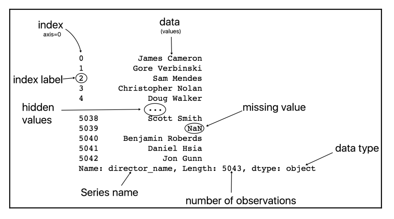
`pd.Series`数据结构解释,这里包含了名字。
`Name: director_name`和`movie['director_name']`相对。
等价于`movie['director_name'].name`
movie[‘director_name’].name ‘director_name’
刚才是
`pd.DataFrame`
$\to$
`pd.Series`
,
现在是
`pd.DataFrame`
$\gets$
`pd.Series`
。
movie[‘director_name’].to_frame() director_name 0 James Cameron 1 Gore Verbinski 2 Sam Mendes 3 Christopher Nolan 4 Doug Walker
`dir(pd.Series)`是list。
`set(dir(pd.Series))`是dict。
len(set(dir(pd.Series))) 455 len(set(dir(pd.DataFrame))) 462 len( set(dir(pd.DataFrame)) & set(dir(pd.Series)) ) 391
有391个attr一起分享!因此接下来直接用`pd.Series`来讲就好了,可以相信很多`pd.DataFrame`类似的。

```
library(DiagrammeR)
grViz(
digraph dot {

graph [layout = dot]

node [shape = egg,
      style = filled,
      color = darkgreen,
      fontsize = 12,
      fontname = Helvetica,
      fontcolor = white,
      # label = ''
]

a [label = 'pd.DataFrame()\npd.Series()']
b [label = 'value_counts\n各level和count']
c [label = 'pctg']
d [label = 'size\nshape']
e [label = 'count']
f [label = 'notnull.sum()']
g [label = 'isnull.sum()']
h [label = 'hasnans\n是否有NaN']
i [label = '.mean\n缺失率']
j [label = '.dropna()']
k [label = '.fillna()']

edge [
      color = darkgreen,
      fontsize = 9,
      fontname = Helvetica,
      fontcolor = dodgerblue,
      label = '']

a -> {b d}
b -> c [label = 'normalize']
d -> e [label = 'x NaN']
e -> f [label = '=']
f -> g
g -> h -> i -> {j k}

}")
pd.Series主要参数
movie['director_name'].value_counts().head()
Steven Spielberg    26
Woody Allen         22
Martin Scorsese     20
Clint Eastwood      20
Ridley Scott        16
Name: director_name, dtype: int64

movie['actor_1_facebook_likes'].value_counts(normalize = True).head()
1000.0     0.088816
11000.0    0.041964
2000.0     0.038501
3000.0     0.030556
12000.0    0.026686
Name: actor_1_facebook_likes, dtype: float64
value_counts()是一个pd.Series看造型。
功能类似于R的group_by加count()。
movie['director_name'].size
movie['director_name'].shape
4916
(4916,)

movie['director_name'].count()
4814
不考虑NaN。
movie['actor_1_facebook_likes'].min()
movie['actor_1_facebook_likes'].max()
movie['actor_1_facebook_likes'].std()
movie['actor_1_facebook_likes'].mean()
movie['actor_1_facebook_likes'].median()
movie['actor_1_facebook_likes'].sum()

movie['director_name'].describe()
count                 4814
unique                2397
top       Steven Spielberg
freq                    26
Name: director_name, dtype: object
是一个pd.Series看造型。
count      4909.000000
mean       6494.488491
std       15106.986884
min           0.000000
25%         607.000000
50%         982.000000
75%       11000.000000
max      640000.000000
Name: actor_1_facebook_likes, dtype: float64
分类变量和连续变量不太一样,但是还是skimr的套路。
开始统计点的东西了。
movie['actor_1_facebook_likes'].quantile([0.1,0.2])
0.1    240.0
0.2    510.0
Name: actor_1_facebook_likes, dtype: float64

movie['actor_1_facebook_likes'].isnull().head()
0    False
1    False
2    False
3    False
4    False
Name: actor_1_facebook_likes, dtype: bool
movie['actor_1_facebook_likes'].isnull().sum()
movie['actor_1_facebook_likes'].hasnans
True
.mean()可以看缺失率。
应该做一个cheatsheet。
movie['actor_1_facebook_likes'].notnull().head()
0    True
1    True
2    True
3    True
4    True
Name: actor_1_facebook_likes, dtype: bool

movie['actor_1_facebook_likes'].fillna(movie['actor_1_facebook_likes'].median())
movie['actor_1_facebook_likes'].dropna().head()

0     1000.0
1    40000.0
2    11000.0
3    27000.0
4      131.0
Name: actor_1_facebook_likes, dtype: float64
到此为止,不可能轻视pd.Series了,其实还有更多。 keep going。
对pd.Series运算
movie['actor_1_facebook_likes'] + 2
movie['actor_1_facebook_likes'] * 2
(movie['actor_1_facebook_likes']// 2).head()

imdb_score.add(1)             # imdb_score + 1
imdb_score.mul(2.5)           # imdb_score * 2.5
imdb_score.floordiv(7)        # imdb_score // 7
imdb_score.gt(7)              # imdb_score > 7
director.eq('James Cameron')  # director == 'James Cameron'
方便method chaining
对pd.Seriesmethod chaining的理解
movie['actor_1_facebook_likes'].fillna(0).astype(int).head()
0     1000
1    40000
2    11000
3    27000
4      131
Name: actor_1_facebook_likes, dtype: int64
```{r echo=FALSE, message=FALSE, warning=FALSE} library(DiagrammeR) grViz( digraph dot {
graph [layout = dot]
node [shape = egg, style = filled, color = darkgreen, fontsize = 12, fontname = Helvetica, fontcolor = white, # label = ‘’]
a [label = ‘默认index’] b [label = ‘特定index’] c [label = ‘rename index’] d [label = ‘add/drop’]
edge [ color = darkgreen, fontsize = 9, fontname = Helvetica, fontcolor = dodgerblue, label = ‘’]
a -> b [label = ‘.set_index(varsName)’] a -> b [label = ‘pd.read_csv + \nindex_col = varsName’] b -> a [label = ‘reset_index()’] a -> c [label = ‘.rename + dict’] a -> c [label = ‘.tolist() + list[0] = …’] a -> d [label = ‘[…] = …’] a -> d [label = ‘.insert()\n自定义位置’] a -> d [label = ‘.drop()’]
}")
## 重设index
movie2 = pd.read_csv(“data/movie.csv”) movie2.set_index(“movie_title”).head()
or
pd.read_csv(“data/movie.csv”, index_col = “movie_title”).head()
复原
pd.read_csv(“data/movie.csv”, index_col = “movie_title”).reset_index().head()
## 给个别index重命名
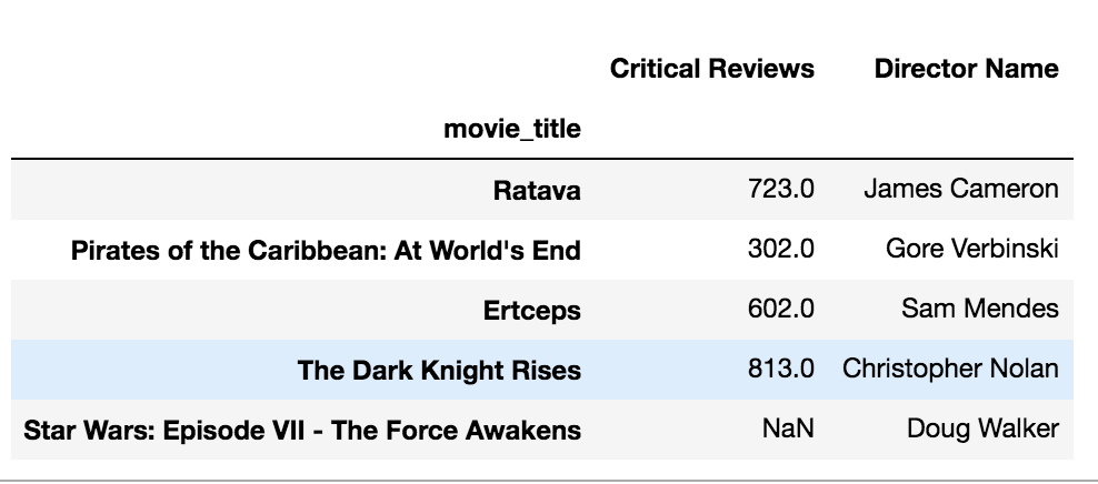
movie = pd.read_csv(‘data/movie.csv’, index_col=‘movie_title’) idx_name = { ‘Avatar’:‘Ratava’, ‘Spectre’: ‘Ertceps’ } col_rename = { ‘director_name’:‘Director Name’, ’num_critic_for_reviews’: ‘Critical Reviews’ } movie_renamed = movie.rename(index = idx_name, columns = col_rename) movie_renamed[[‘Critical Reviews’,‘Director Name’]].head()
用字典格式。
old keys and new values。
用python list来进行修改。
movie = pd.read_csv(‘data/movie.csv’, index_col=‘movie_title’) print type(movie.index) print type(movie.index.tolist()) print type(movie.columns) print type(movie.columns.tolist()) index_list = movie.index.tolist() column_list = movie.columns.tolist() index_list[0] = ‘Ratava’ index_list[1] = ‘Ertceps’ column_list[1] = ‘Director Name’ column_list[2] = ‘Critical Reviews’ print index_list[0:2] print column_list[1:3]
<class ‘pandas.core.indexes.base.Index’> <type ’list’> <class ‘pandas.core.indexes.base.Index’> <type ’list’> [‘Ratava’, ‘Ertceps’] [‘Director Name’, ‘Critical Reviews’]
movie.index = index_list movie.columns = column_list
显然还是`rename`简单,但是`.tolist()`可以学习一下。

## 增删列

就是加入`pd.Series`,Calling Series method。
movie = pd.read_csv(‘data/movie.csv’) movie[‘has_seen’] = 0 movie.columns.values[-1] ‘has_seen’
下面进行`pd.Series`计算。
movie[‘actor_director_facebook_likes’] =
(movie[‘actor_1_facebook_likes’] + movie[‘actor_2_facebook_likes’] + movie[‘actor_3_facebook_likes’] + movie[‘director_facebook_likes’])
检查是否有空值。
movie[‘actor_director_facebook_likes’].isnull().sum()
空值覆盖。
movie[‘actor_director_facebook_likes’] =
movie[‘actor_director_facebook_likes’].fillna(0)
movie[‘is_cast_likes_more’] =
(movie[‘cast_total_facebook_likes’] >= movie[‘actor_director_facebook_likes’])
movie[‘is_cast_likes_more’].all()
现在`'is_cast_likes_more'`是T/F值,我们可以检查是否
__全部是T__,用`.all()`。
但是`any`是只要满足一个就行,
两者相对。


最后T这列。
movie = movie.drop(‘actor_director_facebook_likes’, axis=‘columns’)
`.drop`默认是用index name。
`axis='columns'`是对列。

或者
del movie[‘actor_director_facebook_likes’]
## 插入一列还自定义位置
movie = pd.read_csv(‘data/movie.csv’) print movie.columns.get_loc(“gross”) print movie.columns.get_loc(“gross”) + 1 movie_insert =
movie.insert(loc = movie.columns.get_loc(“gross”) + 1, column = ‘profit’, value = movie[‘gross’] - movie[‘budget’] ) print movie.columns[[8,9]] 8 9 Index([u’gross’, u’profit’], dtype=‘object’)
因此,这样就不会打乱顺序。


加入结构图,第一章,完成。

# 第二章

## 多选列和tuple
movie[[“color”,“director_name”]].head()
color director_name 0 Color James Cameron 1 Color Gore Verbinski 2 Color Sam Mendes 3 Color Christopher Nolan 4 NaN Doug Walker
这里可以使用`[]`,但是不能使用`()`,因为
tuple1 = “color”,“director_name (“color”,“director_name”) == tuple1 True
因此本质上tuple不是一个list,而是一个没有边界的一串数字,是不能够接受的。

## python中的`select_if`和根据变量属性选择
movie = pd.read_csv(“data/movie.csv”, index_col=‘movie_title’) print movie.get_dtype_counts()
float64 13 int64 3 object 11 dtype: int64
print movie.select_dtypes(include = [‘int’]).head()
num_voted_users \
movie_title
Avatar 886204
Pirates of the Caribbean: At World’s End 471220
Spectre 275868
The Dark Knight Rises 1144337
Star Wars: Episode VII - The Force Awakens 8
cast_total_facebook_likes \
movie_title
Avatar 4834
Pirates of the Caribbean: At World’s End 48350
Spectre 11700
The Dark Knight Rises 106759
Star Wars: Episode VII - The Force Awakens 143
movie_facebook_likes
movie_title
Avatar 33000
Pirates of the Caribbean: At World’s End 0
Spectre 85000
The Dark Knight Rises 164000
Star Wars: Episode VII - The Force Awakens 0
珍惜时间,focus on what matter.


[`print movie.select_dtypes(exclude=[object]).head()`](https://stackoverflow.com/questions/21271581/selecting-pandas-columns-by-dtype)
也是可以的,因此`include/exclude`后,包括`""`和直接写词都可以。

[`help(pd.DataFrame.select_dtypes)`中表示,](https://zhuanlan.zhihu.com/p/28085204)。
include, exclude : scalar or list-like A selection of dtypes or strings to be included/excluded. At least one of these parameters must be supplied.
movie.filter(like = “facebook”).head()
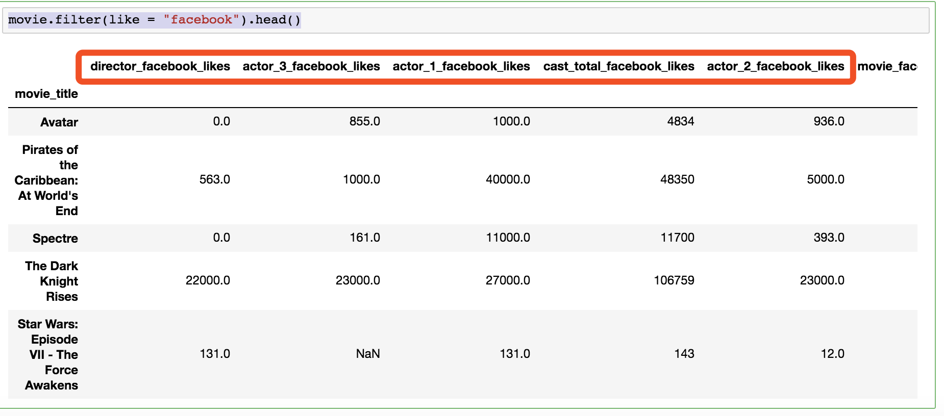
filter(self, items=None, like=None, regex=None, axis=None) unbound pandas.core.frame.DataFrame method Subset rows or columns of dataframe according to labels in the specified index.
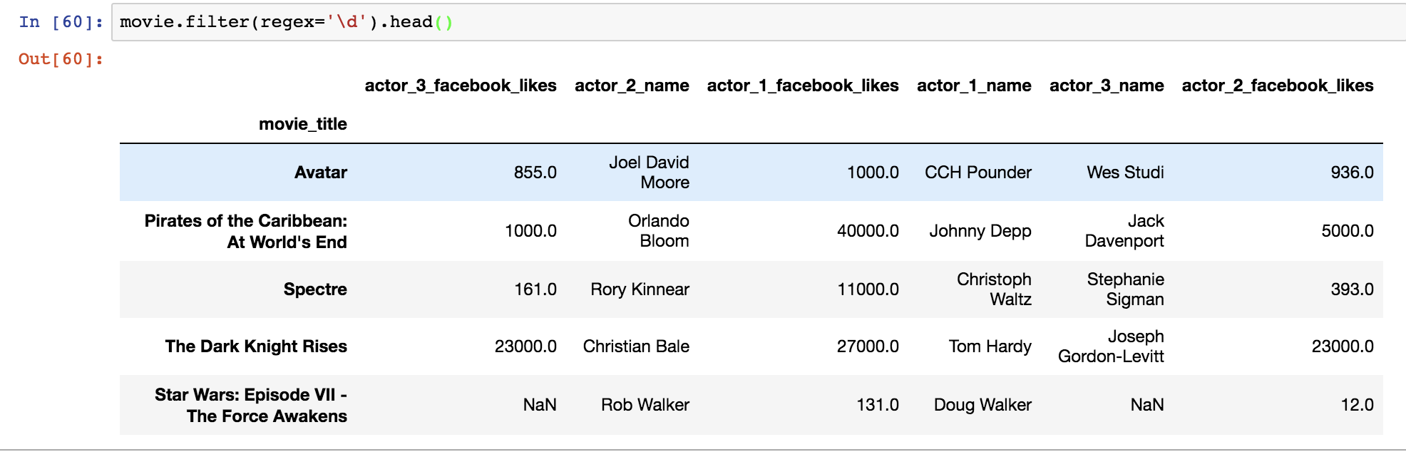
movie.filter(regex=’\d’).head()
## 自定义分组、排序变量
直接选择好,相加就好。
movie = pd.read_csv(“data/movie.csv”) print movie.columns disc_core = [‘movie_title’, ’title_year’, ‘content_rating’, ‘genres’] disc_people = [‘director_name’, ‘actor_1_name’, ‘actor_2_name’, ‘actor_3_name’] disc_other = [‘color’, ‘country’, ’language’, ‘plot_keywords’, ‘movie_imdb_link’] cont_fb = [‘director_facebook_likes’, ‘actor_1_facebook_likes’, ‘actor_2_facebook_likes’, ‘actor_3_facebook_likes’, ‘cast_total_facebook_likes’, ‘movie_facebook_likes’] cont_finance = [‘budget’, ‘gross’] cont_num_reviews = [’num_voted_users’, ’num_user_for_reviews’, ’num_critic_for_reviews’] cont_other = [‘imdb_score’, ‘duration’, ‘aspect_ratio’, ‘facenumber_in_poster’] new_col_order = disc_core + disc_people +
disc_other + cont_fb +
cont_finance + cont_num_reviews +
cont_other
验证这次reorder后,变量没漏。
set(movie.columns) == set(new_col_order) True
## 了解一个表的数据结构 dive in
movie = pd.read_csv(‘data/movie.csv’) print movie.size print movie.shape print len(movie) print len(movie.columns) print len(movie)*len(movie.columns)
137648 (4916, 28) 4916 28 137648
print movie.count().head() # 之前是pd.Series所以只反馈一列,这里是所有变量。 print movie.min().head() print movie.describe().head()
color 4897 director_name 4814 num_critic_for_reviews 4867 duration 4901 director_facebook_likes 4814 dtype: int64 color inf director_name inf num_critic_for_reviews 1 duration 7 director_facebook_likes 0 dtype: object num_critic_for_reviews duration director_facebook_likes
count 4867.000000 4901.000000 4814.000000
mean 137.988905 107.090798 691.014541
std 120.239379 25.286015 2832.954125
min 1.000000 7.000000 0.000000
25% 49.000000 93.000000 7.000000
actor_3_facebook_likes actor_1_facebook_likes gross \
count 4893.000000 4909.000000 4.054000e+03
mean 631.276313 6494.488491 4.764451e+07
std 1625.874802 15106.986884 6.737255e+07
min 0.000000 0.000000 1.620000e+02
25% 132.000000 607.000000 5.019656e+06
num_voted_users cast_total_facebook_likes facenumber_in_poster \
count 4916.000000 4916.000000 4903.000000
mean 82644.924939 9579.815907 1.377320
std 138322.162547 18164.316990 2.023826
min 5.000000 0.000000 0.000000
25% 8361.750000 1394.750000 0.000000
num_user_for_reviews budget title_year \
count 4895.000000 4.432000e+03 4810.000000
mean 267.668846 3.654749e+07 2002.447609
std 372.934839 1.002427e+08 12.453977
min 1.000000 2.180000e+02 1916.000000
25% 64.000000 6.000000e+06 1999.000000
actor_2_facebook_likes imdb_score aspect_ratio movie_facebook_likes
count 4903.000000 4916.000000 4590.000000 4916.000000
mean 1621.923516 6.437429 2.222349 7348.294142
std 4011.299523 1.127802 1.402940 19206.016458
min 0.000000 1.600000 1.180000 0.000000
25% 277.000000 5.800000 1.850000 0.000000
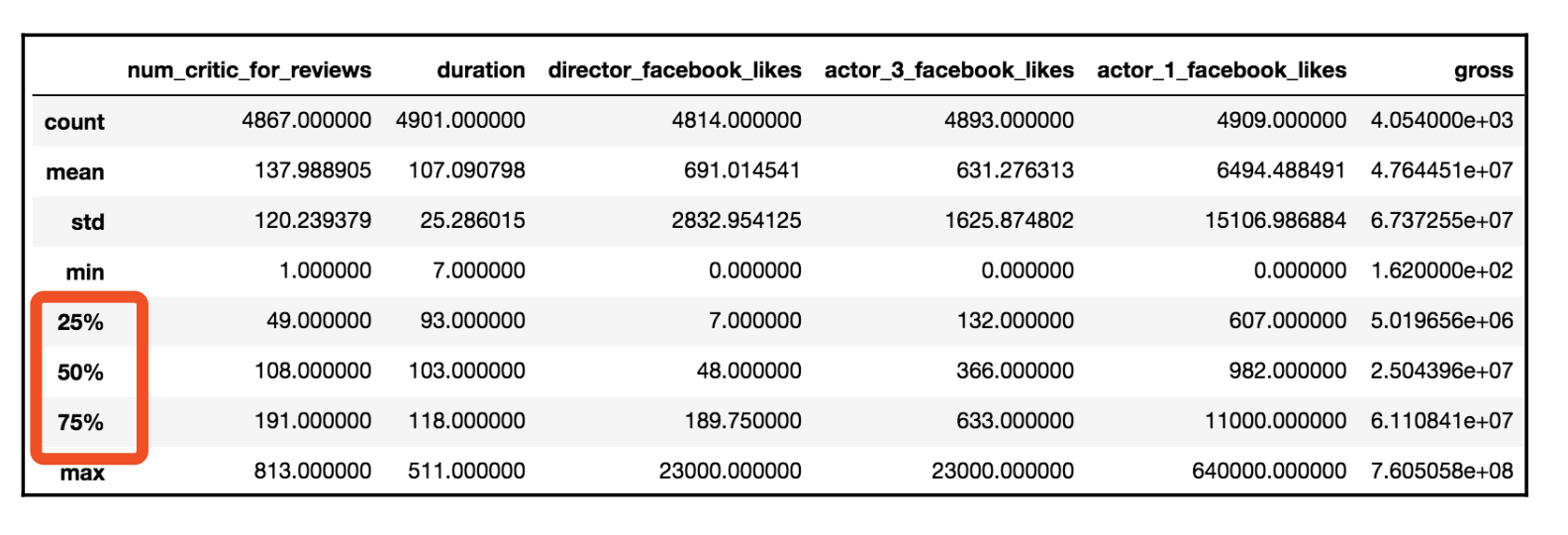
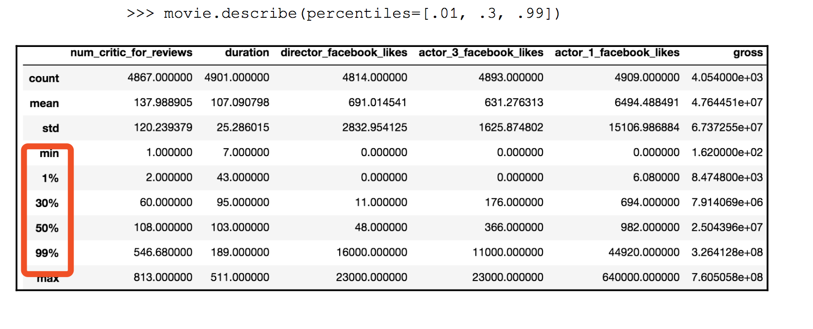
这里可以自定义pecentile。
print movie.describe(percentiles=[0.11,0.99]).head(n=7)
print movie.min().head() print movie.min(skipna=False).head()
color inf director_name inf num_critic_for_reviews 1 duration 7 director_facebook_likes 0 dtype: object color NaN director_name NaN num_critic_for_reviews 1 duration 43 director_facebook_likes 0 dtype: object
显然`skipna=False`反馈了分类变量为`inf`,有缺失值的连续变量反馈为`NaN`。

## 整合


## 缺失值探查用method chaining
print movie.isnull().head() # 一个全是T/F的pd.DataFrame print movie.isnull().sum().head() # 一个累计值的pd.Series print movie.isnull().sum().sum() # 一个累计值
`help(pd.Series.any)`
Return __whether__ any element is __True__ over __requested__ axis
反馈是否exist。
print movie.isnull().any().head() # 对列检验 print movie.isnull().any().any() # 对列的列,也就是DataFrame检验 color True director_name True num_critic_for_reviews True duration True director_facebook_likes True dtype: bool True
这本书,每个知识点不是糊过去,看出来是真的非常懂,因此写的非常好,看完后,对pandas的理解会非常深,而不不会有dplyr那种瓶颈的感觉。

## 查看每列最多频率分类
movie.get_dtype_counts() # 不print了,因为只是探查,验证object是否存在 movie.select_dtypes(include =[object]).min() # inf表示有空置,需要进行替换 movie.select_dtypes(include =[object]).fillna(’’).min() movie.select_dtypes(include =[object])
.fillna(’’)
.min() # 为了readable
color
director_name
actor_2_name
genres Action actor_1_name
movie_title #Horror actor_3_name
plot_keywords
movie_imdb_link http://www.imdb.com/title/tt0006864/?ref_=fn_t… language
country
content_rating
dtype: object
## 展示数据只有两位小数点
college = pd.read_csv(‘data/college.csv’) # college + 5 #会报错,因为有非int的变量 college_ugds_ = college.filter(like=‘UGDS_’) + 0.00501 (college_ugds_ + .00501) // .01 # 仿round函数 (college_ugds_ + .00501) // .01 /100 #先乘取整数,后除,因此保留2位小数 college_ugds_.round(2) # 等价,如果数据表是全int的,全部保留两位小数,展示数据的时候很必要。 college_ugds_.round(2).head()
college_ugds_.round(2).equals( ((college_ugds_ + .00501) // .01 /100) ) True
## 注意float值
.045 + .005 0.049999999999999996
print .045 + .005 print .045 + .00501 0.05 0.05001
因此加的时候,应该加`.00501`而非`.005`,因为`print`都看不出来。

## 缺失值理解
import numpy as np print np.nan == np.nan print None == None print np.nan > 5 print 5 > np.nan print np.nan != 5
False True False False True
`pandas`使用`np.nan`作为缺失值的表达,而非`None`。
`np.nan`连自身都不相等。
所以用`data[data['x'] == np.nan]`是不靠谱的。
## 检验两表相等
由上得知,不能用`.eq`,没有用,而是用`.equals`。
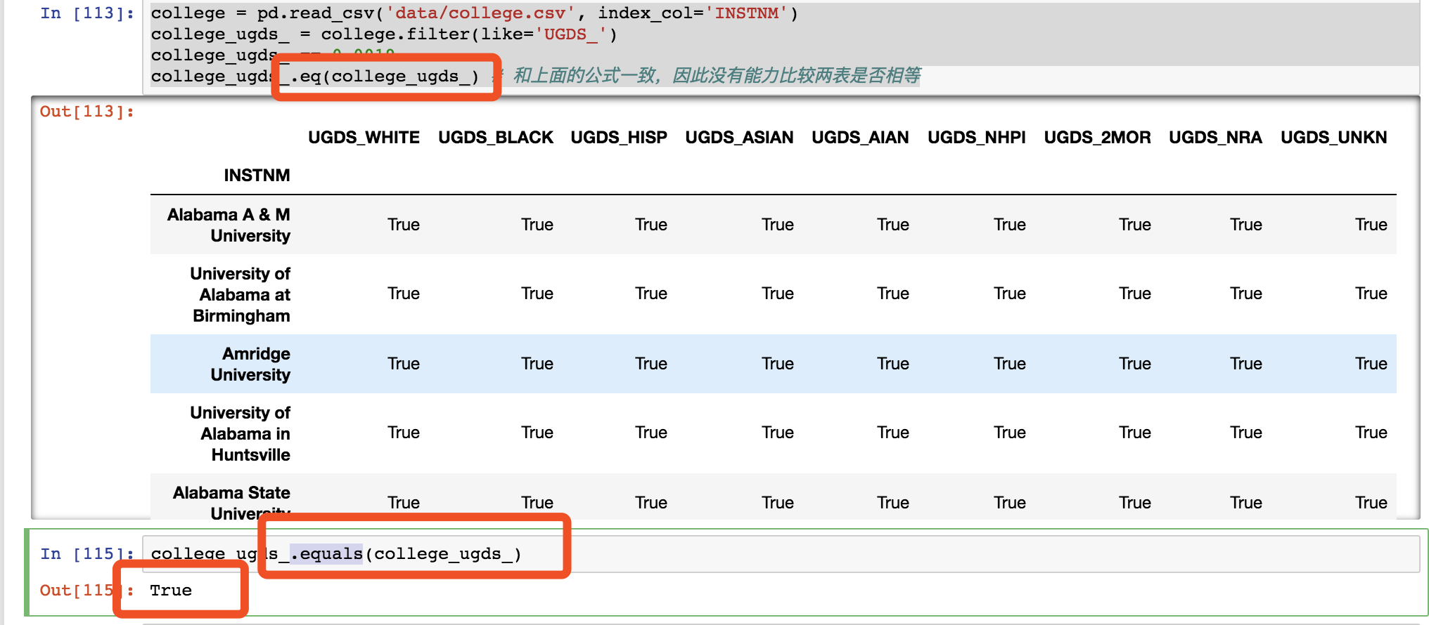
from pandas.testing import assert_frame_equal # 断言frame是否相等 print assert_frame_equal(college_ugds_,college_ugds_) None
如果回复`None`那么就是对的了。

## 转置和`axis`

一般`axis=0`或者`axis='index'`这是默认的,
特别地,可以设置,
`axis=1`或者`axis='columns'`这是默认的。

__一般`axis=0`或者`axis='index'`这是默认的,__
这句话是一直发生的,比如,我举个例子。
college = pd.read_csv(‘data/college.csv’, index_col=‘INSTNM’) college.filter(like = “UGDS_”).count() UGDS_WHITE 6874 UGDS_BLACK 6874 UGDS_HISP 6874 UGDS_ASIAN 6874 UGDS_AIAN 6874 UGDS_NHPI 6874 UGDS_2MOR 6874 UGDS_NRA 6874 UGDS_UNKN 6874 dtype: int64
这里的`.count()`反馈非空值的数量,注意是根据index扫描而得,类似于
college = pd.read_csv(‘data/college.csv’, index_col=‘INSTNM’) college.filter(like = “UGDS_”).count() from pandas.testing import assert_series_equal print assert_series_equal( college.filter(like = “UGDS_”).count(), college.filter(like = “UGDS_”).count(axis = 0) ) print assert_series_equal( college.filter(like = “UGDS_”).count(), college.filter(like = “UGDS_”).count(axis = ‘index’) )
None None
所以
college_ugds_.count(axis = 1).head() INSTNM Alabama A & M University 9 University of Alabama at Birmingham 9 Amridge University 9 University of Alabama in Huntsville 9 Alabama State University 9 dtype: int64
还有`.sum()`
college_ugds_.sum(axis = 1).head() INSTNM Alabama A & M University 1.0000 University of Alabama at Birmingham 0.9999 Amridge University 1.0000 University of Alabama in Huntsville 1.0000 Alabama State University 1.0000 dtype: float64
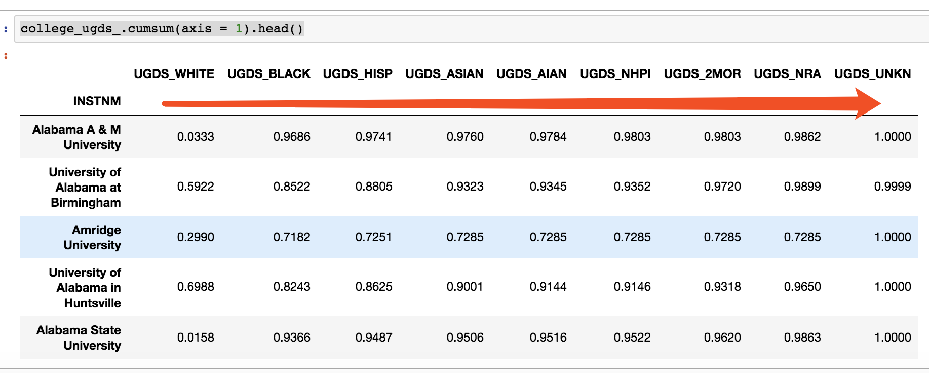
还有`.cumsum()`
college_ugds_.cumsum(axis = 1).head()
## 排序
`\`后面不能有空格和`#`。
college = pd.read_csv(‘data/college.csv’, index_col=‘INSTNM’) college_ugds_ = college.filter(like=‘UGDS_’) college_ugds_.isnull()
.sum(axis = 1)
.sort_values(ascending = False)
.head()
INSTNM Excel Learning Center-San Antonio South 9 Philadelphia College of Osteopathic Medicine 9 Assemblies of God Theological Seminary 9 Episcopal Divinity School 9 Phillips Graduate Institute 9 dtype: int64
college_ugds_.dropna(how=‘all’)
.isnull()
.sum() UGDS_WHITE 0 UGDS_BLACK 0 UGDS_HISP 0 UGDS_ASIAN 0 UGDS_AIAN 0 UGDS_NHPI 0 UGDS_2MOR 0 UGDS_NRA 0 UGDS_UNKN 0 dtype: int64
`how='all'`表示全部都要是`np.nan`的才T掉。
college_ugds_.ge(.15)
.sum(axis = ‘columns’)
.head() INSTNM Alabama A & M University 1 University of Alabama at Birmingham 2 Amridge University 3 University of Alabama in Huntsville 1 Alabama State University 1 dtype: int64
这里不需要gather函数,直接对整个表进行运算。
college_ugds_.ge(.15)
.sum(axis = ‘columns’)
.value_counts() 1 3042 2 2884 3 876 0 668 4 63 5 2 dtype: int64
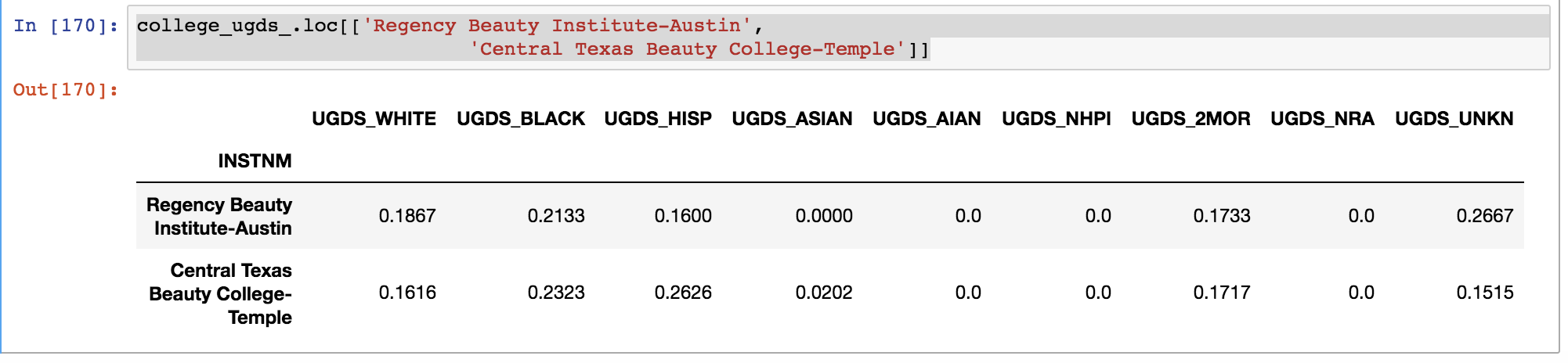
终于知道为什么要用`loc`因为这里的默认是对行不是列。
college_ugds_.loc[[‘Regency Beauty Institute-Austin’, ‘Central Texas Beauty College-Temple’]]
## `all`和`any`的活用
college_ugds_ > 0.01 # 一张表 (college_ugds_ > 0.01).all(axis=1) #一行都要满足,也就是说,一个学校每个种族比例要大于0.01 (college_ugds_ > 0.01).all(axis=1).any() #是否有这样的学校呢,只要有一个,就反馈True
# 第三章 EDA


马上开始第三章!

## 路径

认识dataset。
metadata = data about data。
建议一个研究路径。

```
library(DiagrammeR)
grViz(
digraph dot {

graph [layout = dot]

node [shape = egg,
      style = filled,
      color = darkgreen,
      fontsize = 12,
      fontname = Helvetica,
      fontcolor = white,
      # label = ''
]

a [label = '.head()']
b [label = '.shape\n(nrow,ncol)']
c [label = '.info()\n']
d [label = '.get_dtype_counts()\nfor include']
e [label = '.describe(include = [...]).T']

edge [
      color = darkgreen,
      fontsize = 9,
      fontname = Helvetica,
      fontcolor = dodgerblue,
      label = '']

a -> b
b -> {c d}
d -> e

}")

print college.shape
print college.info()
print college.get_dtype_counts()

import numpy as np
college.describe(include = [np.number]).T.head()
# np.number 就代表全部了,不需要每次去记录float还是int累。
college.describe(include = [np.object,pd.Categorical]).T
# np.object, pd.Categorical 就代表全部了,不需要每次去记录string了。
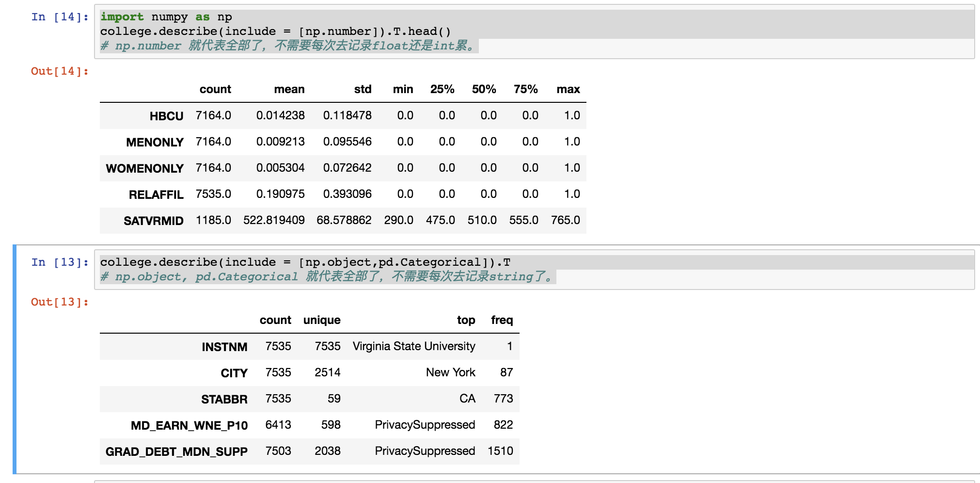
这么复杂没有必要。
college.describe(include = [np.number],
                percentiles = [0.1,0.2,0.3,0.4]

                ).T.head()
改变数据表类型降低表内存
college = pd.read_csv('data/college.csv')
different_cols = ['RELAFFIL', 'SATMTMID', 'CURROPER',
                                  'INSTNM', 'STABBR']
col2 = college.loc[:, different_cols]
print col2.head()

   RELAFFIL  SATMTMID  CURROPER                               INSTNM STABBR
0         0     420.0         1             Alabama A & M University     AL
1         0     565.0         1  University of Alabama at Birmingham     AL
2         1       NaN         1                   Amridge University     AL
3         0     590.0         1  University of Alabama in Huntsville     AL
4         0     430.0         1             Alabama State University     AL

print type(col2.dtypes.to_frame)
print type(col2.memory_usage(deep=True).to_frame)
因此需要进行pd.Series。
print pd.concat(
[pd.Series(col2.dtypes),
pd.Series(col2.memory_usage(deep=True))],
    axis = 'columns'
).sort_values(by = 1,ascending = False)
这里by = 1因为名字是数字。
                0       1
INSTNM     object  569181
STABBR     object  354145
CURROPER    int64   60280
RELAFFIL    int64   60280
SATMTMID  float64   60280
Index         NaN      72
.memory_usage用来提取内存。
col2.RELAFFIL = col2.RELAFFIL.astype(np.int8)

print col2.RELAFFIL.head()
col2.RELAFFIL = col2.RELAFFIL.astype(np.int8)
0    0
1    0
2    1
3    0
4    0
Name: RELAFFIL, dtype: int8
因此调整到np.int8,因为只有0和1.
print col2.select_dtypes(include = [object]).nunique()
col2.STABBR = col2.STABBR.astype('category')
INSTNM    7535
STABBR      59
dtype: int64
STABBR才有50个分类。
college = pd.read_csv('data/college.csv')
different_cols = ['RELAFFIL', 'SATMTMID', 'CURROPER',
                                  'INSTNM', 'STABBR']
col2 = college.loc[:, different_cols]
oldone = col2.memory_usage(deep=True)
col2.RELAFFIL = col2.RELAFFIL.astype(np.int8)
col2.STABBR = col2.STABBR.astype('category')
newone = col2.memory_usage(deep=True)
oldone/newone
Index        1.000000
RELAFFIL     8.000000
SATMTMID     1.000000
CURROPER     1.000000
INSTNM       1.000000
STABBR      27.521371
dtype: float64
这是改良的结果。
nlargest
就是sort_values之间的复用。
movie = pd.read_csv('data/movie.csv')
movie2 = movie[['movie_title', 'imdb_score', 'budget']]
movie2.nlargest(100,'imdb_score').nsmallest(5,'budget')

               movie_title  imdb_score    budget
4804        Butterfly Girl         8.7  180000.0
4801    Children of Heaven         8.5  180000.0
4706          12 Angry Men         8.9  350000.0
4550          A Separation         8.4  500000.0
4636  The Other Dream Team         8.4  500000.0
imdb_score top 100中,budgettop5低的。
保留每组最高分
movie = pd.read_csv('data/movie.csv')
movie2 = movie[['movie_title', 'title_year', 'imdb_score']]
movie2.sort_values(['title_year','imdb_score'], ascending=[True,False])\
    .drop_duplicates(subset = 'title_year').head()

                                           movie_title  title_year  imdb_score
4695  Intolerance: Love's Struggle Throughout the Ages      1916.0         8.0
4833                    Over the Hill to the Poorhouse      1920.0         4.8
4767                                    The Big Parade      1925.0         8.3
2694                                        Metropolis      1927.0         8.3
4555                                     Pandora's Box      1929.0         8.0
movie2.sort_values中,list和ascending都是可以自定义的。 .drop_duplicates(subset = 'title_year')类似于group_by()。
nlargest/nsmallest和sort_value的一点区别
print movie2.nlargest(100, 'imdb_score').tail()
                movie_title  imdb_score     budget
4023                 Oldboy         8.4  3000000.0
4163  To Kill a Mockingbird         8.4  2000000.0
4395         Reservoir Dogs         8.4  1200000.0
4550           A Separation         8.4   500000.0
4636   The Other Dream Team         8.4   500000.0

print movie2.sort_values('imdb_score', ascending=False) \
             .head(100).tail()
                                  movie_title  imdb_score      budget
3799                     Anne of Green Gables         8.4         NaN
3777                      Requiem for a Dream         8.4   4500000.0
3935  Batman: The Dark Knight Returns, Part 2         8.4   3500000.0
4636                     The Other Dream Team         8.4    500000.0
2455                                   Aliens         8.4  18500000.0

print pd.merge(
    movie2.nlargest(100, 'imdb_score').tail(),
    movie2.sort_values('imdb_score', ascending=False) \
             .head(100).tail()

)

            movie_title  imdb_score    budget
0  The Other Dream Team         8.4  500000.0
只有一个类似为什么?
因为
print (movie2.imdb_score > 8.4).sum()
print (movie2.imdb_score == 8.4).sum()
print (movie2.imdb_score < 8.4).sum()
72
29
4815
movie2.imdb_score == 8.4数量太多了。
cummax函数使用
股票市场有stop order,就是说如果100块买入一只股票,当跌到90块时强制卖出。 这时候10%的比例。 我们假设这个比例不变。 当估计上涨到120块时,强制卖出价变为r 120*0.9元。 因此当从120块跌到110块时,强制卖出价还是r 120*0.9元。 因此这就是cummax的思想。
import pandas_datareader as pdr
tsla = pdr.DataReader('tsla', data_source='google',
                                      start='2017-1-1')
(tsla.Close.cummax() * 0.9).head(8)

Date
2017-01-03    195.291
2017-01-04    204.291
2017-01-05    204.291
2017-01-06    206.109
2017-01-09    208.152
2017-01-10    208.152
2017-01-11    208.152
2017-01-12    208.152
Name: Close, dtype: float64
第四章 subset selecting
pandas是从numpy中派生的, 给np.array加index和columns。 这也说明了,为什么pd.Dataframe的index、columns和values本质是np。
indexing operator & indexer
but the primary function of the indexing operator is actually to select DataFrame columns.
说的好!
indexing operator顾名思义就是加减乘除这种,所以是pd.Series(...)[]中的[],然而loc[]就是indexer了。
np.random.seed(1)
# help(np.random.choice)
# choice(a, size=None, replace=True, p=None)

print city.loc[
    list(np.random.choice(city.index, 4))
]

                                                 CITY
INSTNM
Northwest HVAC/R Training Center              Spokane
California State University-Dominguez Hills    Carson
Lower Columbia College                       Longview
Southwest Acupuncture College-Boulder         Boulder
string选择和序号在loc
print city.loc[
    'Alabama State University':
    'Reid State Technical College':
    10
]

                                          CITY
INSTNM
Alabama State University            Montgomery
Enterprise State Community College  Enterprise
Heritage Christian University         Florence
Marion Military Institute               Marion
Reid State Technical College         Evergreen

print city.iloc[[3]]
print city.iloc[3]
print type(city.iloc[[3]])
print type(city.iloc[3])

INSTNM
University of Alabama in Huntsville    Huntsville
Name: CITY, dtype: object
Huntsville
<class 'pandas.core.series.Series'>
<type 'str'>
所以[[d:]]的形式都不会改变结构,也就是说, frame还是frame,series还是series。
从frame拿一个row
college = pd.read_csv('data/college.csv', index_col='INSTNM')
college.head()
print college.iloc[60].head()
print type(college.iloc[60])
# 降维为Series

print type(college.iloc[99:102])
# 注意这种[a:b]其实也是frame,特点。
从frame拿行列
college = pd.read_csv('data/college.csv', index_col='INSTNM')
print college.iloc[:,[-4]].head(n=6)
print college.iloc[5,-4]
# 位置精确

print college.iloc[90:80:-2, 5]
# 这也说明了a:b可以保持frame,
# a>b,c<0

INSTNM
Empire Beauty School-Flagstaff     0
Charles of Italy Beauty College    0
Central Arizona College            0
University of Arizona              0
Arizona State University-Tempe     0
Name: RELAFFIL, dtype: int64
.loc和.iloc混用
college = pd.read_csv('data/college.csv', index_col='INSTNM')

from pandas.testing import assert_frame_equal
print assert_frame_equal(

college.iloc[:5,
            college.columns.get_loc('UGDS_WHITE'):
            college.columns.get_loc('UGDS_UNKN') + 1
            ]
    ,
college.iloc[:5,:].loc[:,'UGDS_WHITE':'UGDS_UNKN']
)
# 显然两个都是frame,这里就不解释了。
.at和.iat迅速取用单值
college = pd.read_csv('data/college.csv', index_col='INSTNM')
cn = 'Texas A & M University-College Station'
print college.loc[cn, 'UGDS_WHITE']
print college.at[cn, 'UGDS_WHITE']
# 因此反馈值,应该是一个值,而非frame或者series。
%timeit college.loc[cn, 'UGDS_WHITE']
%timeit college.at[cn, 'UGDS_WHITE']

0.661
0.661
The slowest run took 6.27 times longer than the fastest. This could mean that an intermediate result is being cached.
100000 loops, best of 3: 12 µs per loop

The slowest run took 4.55 times longer than the fastest. This could mean that an intermediate result is being cached.
100000 loops, best of 3: 7.71 µs per loop
但是明显.at和.iat很快啊。
按照字母顺序来选择
基本想法就是排个序.sort_index(),就可以像字典一样选取了。
college = pd.read_csv('data/college.csv', index_col='INSTNM')
print college.sort_index().iloc[:,:2].loc["Sp":"Su"].head()

                                    CITY STABBR
INSTNM
Spa Tech Institute-Ipswich       Ipswich     MA
Spa Tech Institute-Plymouth     Plymouth     MA
Spa Tech Institute-Westboro     Westboro     MA
Spa Tech Institute-Westbrook   Westbrook     ME
Spalding University           Louisville     KY
.loc["Sp":"Su"]选择首字母长这样的,但是不包含"Su"。 这是正序,还可以倒序。
print college.sort_index(ascending=False).index.is_monotonic_decreasing
print college.sort_index(ascending=False).index.is_monotonic_increasing
# 检查
True
False

print college.sort_index(ascending=False).loc['E':'B'].head().iloc[:,:2]
                                                  CITY STABBR
INSTNM
Dyersburg State Community College            Dyersburg     TN
Dutchess Community College                Poughkeepsie     NY
Dutchess BOCES-Practical Nursing Program  Poughkeepsie     NY
Durham Technical Community College              Durham     NC
Durham Beauty Academy                           Durham     NC
看可以倒序,但是不包含"E"。
第五章
筛选row
movie_2_hours = movie['duration'] > 120
# 反馈boolean 列。

movie_2_hours.describe()
# 这里就是T/F
# freq 是 top的freq

count      4916
unique        2
top       False
freq       3877
Name: duration, dtype: object

print movie_2_hours.value_counts(normalize=True)
False    0.788649
True     0.211351
Name: duration, dtype: float64
这里证明了。
actor = \
movie.filter(like = 'facebook_likes') \
    .filter(like = 'actor') \
    .iloc[:,1:3]\
    .dropna()
(actor.actor_1_facebook_likes > actor.actor_2_facebook_likes).mean()
#actor.head()
# pd.DataFrame.filter?
# 可以多个filter method chaining
0.977768713033
多个筛选条件
movie = pd.read_csv('data/movie.csv', index_col='movie_title')
movie.head()
(
(movie.imdb_score > 8) &
(movie.content_rating == 'PG-13') &
((movie.title_year < 2000) | (movie.title_year > 2009))
).head()
# and = &
# or = |
# not = ~
把筛选条件应用到frame。
print movie[
    (
    (movie.imdb_score > 8) &
    (movie.content_rating == 'PG-13') &
    ((movie.title_year < 2000) | (movie.title_year > 2009))
    )
].iloc[:,:2].head()

                            color      director_name
movie_title
The Dark Knight Rises       Color  Christopher Nolan
The Avengers                Color        Joss Whedon
Captain America: Civil War  Color      Anthony Russo
Guardians of the Galaxy     Color         James Gunn
Interstellar                Color  Christopher Nolan
用columns筛选快一些
%timeit college[college.STABBR == 'TX']
college2 = college.set_index('STABBR')
%timeit college2.loc['TX']
# 用时更长,因为set_index,本身就是花时间的。
# 但是真正筛选的时候,快很多。

1000 loops, best of 3: 1.12 ms per loop
1000 loops, best of 3: 511 µs per loop

states = ['TX', 'CA', 'NY']
%timeit college[college.STABBR.isin(states)]
%timeit college2.loc[states]
# 但是如果筛选是若干的时候,反而columns的筛选好。
# 综上,我们不可能总是去set_index的,
# 因此,还是推荐用,columns进行筛选。

1000 loops, best of 3: 947 µs per loop
1000 loops, best of 3: 1.55 ms per loop
.isin可以好好用用。 index也就取一个的时候,好用。 但是我觉得这一直是一个很trivial的问题,closed。
合成index
college = pd.read_csv('data/college.csv')
print college.set_index(
college.CITY + ', ' + college.STABBR
).sort_index().head().iloc[:,:2]

                                 INSTNM      CITY
ARTESIA, CA           Angeles Institute   ARTESIA
Aberdeen, SD       Presentation College  Aberdeen
Aberdeen, SD  Northern State University  Aberdeen
Aberdeen, WA       Grays Harbor College  Aberdeen
Abilene, TX   Hardin-Simmons University   Abilene
warning line
slb = pd.read_csv('data/slb_stock.csv', index_col='Date',
                                 parse_dates=['Date'])
slb.Close[
(slb.Close.describe(percentiles=[0.1,0.9]).loc['10%'] < slb.Close) &
(slb.Close.describe(percentiles=[0.1,0.9]).loc['90%'] > slb.Close)
    ]
取outliers,前10%后10%。
累加的index条件
实际上就是产生一列同长度的T/F列,相当于打上了标签,用此在.loc[]上,筛选表。
employee = pd.read_csv('data/employee.csv')
employee.DEPARTMENT.value_counts().head()
employee.GENDER.value_counts()
employee.BASE_SALARY.describe().astype(int)
depts = ['Houston Police Department-HPD',
                         'Houston Fire Department (HFD)']
criteria_dept = employee.DEPARTMENT.isin(depts)
criteria_gender = employee.GENDER == 'Female'
criteria_sal = employee.BASE_SALARY.between(80000, 120000)
criteria_final = (criteria_dept &
                                  criteria_gender &
                                  criteria_sal)
select_columns = ['UNIQUE_ID', 'DEPARTMENT',
                                 'GENDER', 'BASE_SALARY']
print employee.loc[criteria_final, select_columns].head()

     UNIQUE_ID                     DEPARTMENT  GENDER  BASE_SALARY
61          61  Houston Fire Department (HFD)  Female      96668.0
136        136  Houston Police Department-HPD  Female      81239.0
367        367  Houston Police Department-HPD  Female      86534.0
474        474  Houston Police Department-HPD  Female      91181.0
513        513  Houston Police Department-HPD  Female      81239.0
粗略检验连续变量是否符合正态分布
amzn = pd.read_csv('data/amzn_stock.csv', index_col='Date',
                                  parse_dates=['Date'])
amzn_daily_return = amzn.Close.pct_change().dropna()
amzn_daily_return.mean()
amzn_daily_return.std()
((amzn_daily_return - amzn_daily_return.mean()).abs()/amzn_daily_return.std()).lt(1).mean()

# .abs()是为了算在一倍标准差内,有多少样本。
# 这里假设了,1是正态分布的标准差。
# .lt = < 1

pcts = [((amzn_daily_return - amzn_daily_return.mean()).abs()/amzn_daily_return.std()).lt(i).mean() for i in range(1,4)]
# 4是因为开区间。
pcts
[0.78733509234828492, 0.95620052770448549, 0.98469656992084431]
68-95-99.7 这是正态分布的要求, 但是我们拿到的是 78-95.6-98 因此不是正态分布。
print ('{:.3f} fall within 1 standard deviation. '
               '{:.3f} within 2 and {:.3f} within 3'.format(*pcts))
# {:.3f}不是很理解。
0.787 fall within 1 standard deviation. 0.956 within 2 and 0.985 within 3
queryfancy work
但是不适合生产。
depts = ['Houston Police Department-HPD',
                         'Houston Fire Department (HFD)']
select_columns = ['UNIQUE_ID', 'DEPARTMENT',
                                  'GENDER', 'BASE_SALARY']
print employee[select_columns] \
.loc[
    (employee.DEPARTMENT.isin(depts)) &
    (employee.GENDER == 'Female') &
    (employee.BASE_SALARY >= 80000) &
    (employee.BASE_SALARY <= 120000)
].head()
qs = "DEPARTMENT in @depts " \
    "and GENDER == 'Female' " \
    "and 80000 <= BASE_SALARY <= 120000
print employee[select_columns].query(qs).head()
# 外在变量才要加@

%timeit (employee[select_columns].loc[(employee.DEPARTMENT.isin(depts)) & (employee.GENDER == 'Female') &(employee.BASE_SALARY >= 80000) &(employee.BASE_SALARY <= 120000)].head())
%timeit employee[select_columns].query(qs).head()

     UNIQUE_ID                     DEPARTMENT  GENDER  BASE_SALARY
61          61  Houston Fire Department (HFD)  Female      96668.0
136        136  Houston Police Department-HPD  Female      81239.0
367        367  Houston Police Department-HPD  Female      86534.0
474        474  Houston Police Department-HPD  Female      91181.0
513        513  Houston Police Department-HPD  Female      81239.0
100 loops, best of 3: 3.02 ms per loop
100 loops, best of 3: 5.61 ms per loop
显然用queryrun起来很慢,但是呢,简单,可以尝试。 不然boolean太烦了。
top10_depts = employee.DEPARTMENT.value_counts() \
                                        .index[:10].tolist()
employee.DEPARTMENT.value_counts().index[:10].tolist()
# index就是index格式,其中也可以indexing选数字的。
print employee.query(
"DEPARTMENT not in @top10_depts and GENDER == 'Female'
).head()

     UNIQUE_ID                    POSITION_TITLE  \
0            0       ASSISTANT DIRECTOR (EX LVL)
73          73         ADMINISTRATIVE SPECIALIST
96          96     ASSISTANT CITY CONTROLLER III
117        117  SENIOR ASSISTANT CITY ATTORNEY I
146        146              SENIOR STAFF ANALYST

                        DEPARTMENT  BASE_SALARY                       RACE  \
0      Municipal Courts Department     121862.0            Hispanic/Latino
73           Human Resources Dept.      55939.0  Black or African American
96        City Controller's Office      59077.0     Asian/Pacific Islander
117               Legal Department      90957.0  Black or African American
146  Houston Information Tech Svcs      74951.0                      White

    EMPLOYMENT_TYPE  GENDER EMPLOYMENT_STATUS   HIRE_DATE    JOB_DATE
0         Full Time  Female            Active  2006-06-12  2012-10-13
73        Full Time  Female            Active  2011-12-19  2013-11-23
96        Full Time  Female            Active  2013-06-10  2013-06-10
117       Full Time  Female            Active  1998-03-20  2012-07-21
146       Full Time  Female            Active  2014-03-17  2014-03-17
clip和where函数保留原值
movie = pd.read_csv('data/movie.csv', index_col='movie_title')
fb_likes = movie.actor_1_facebook_likes.dropna()
fb_likes.head()
# 某一列。
fb_likes.describe(percentiles=[.1, .25, .5, .75, .9])
fb_likes.where(fb_likes < 20000).head()
# fb_likes还是个列。
# 类似于left join不满足的就NaN
fb_likes.where(fb_likes < 20000,other=20000).where(fb_likes<300,other=300).head()
fb_likes.clip(lower = 300,upper= 20000).head()
fb_likes.clip(lower=300, upper=20000).equals(
fb_likes.where(fb_likes < 20000,other=20000).where(fb_likes<300,other=300)
)

movie_title
Avatar                                         1000.0
Pirates of the Caribbean: At World's End          NaN
Spectre                                       11000.0
The Dark Knight Rises                             NaN
Star Wars: Episode VII - The Force Awakens      131.0
Name: actor_1_facebook_likes, dtype: float64
mask
mask相对于where和clip, 当True时,覆盖那一排都变成NaN了。
movie = pd.read_csv('data/movie.csv', index_col='movie_title')
c1 = movie.title_year > 2010
c2 = movie.title_year.isnull()
criteria = c1 | c2
type(movie.mask(criteria).head())
print movie.mask(criteria).iloc[:,2:4].head()

                                            num_critic_for_reviews  duration
movie_title
Avatar                                                       723.0     178.0
Pirates of the Caribbean: At World's End                     302.0     169.0
Spectre                                                        NaN       NaN
The Dark Knight Rises                                          NaN       NaN
Star Wars: Episode VII - The Force Awakens                     NaN       NaN

movie = pd.read_csv('data/movie.csv', index_col='movie_title')
c1 = movie.title_year >= 2010
c2 = movie.title_year.isnull()
criteria = c1 | c2
type(movie.mask(criteria).head())
movie.mask(criteria).iloc[:,2:4].head()
movie_mask = movie.mask(criteria).dropna(how = 'all')
movie_boolean = movie[movie['title_year'] < 2010]
print movie_mask.equals(movie_boolean)
print movie_mask.shape == movie_boolean.shape
print movie_mask.dtypes ==movie_boolean.dtypes
from pandas.testing import assert_frame_equal
assert_frame_equal(movie_boolean, movie_mask, check_dtype=False)
# 可以不检查变量属性,只比较值。

False
True
color                         True
director_name                 True
num_critic_for_reviews        True
duration                      True
director_facebook_likes       True
actor_3_facebook_likes        True
actor_2_name                  True
actor_1_facebook_likes        True
gross                         True
genres                        True
actor_1_name                  True
num_voted_users              False
cast_total_facebook_likes    False
actor_3_name                  True
facenumber_in_poster          True
plot_keywords                 True
movie_imdb_link               True
num_user_for_reviews          True
language                      True
country                       True
content_rating                True
budget                        True
title_year                    True
actor_2_facebook_likes        True
imdb_score                    True
aspect_ratio                  True
movie_facebook_likes         False
dtype: bool
None
.loc和.iloc的区别
movie = pd.read_csv('data/movie.csv', index_col='movie_title')
c1 = movie['content_rating'] == 'G'
c2 = movie['imdb_score'] < 4
criteria = c1 & c2
movie_loc = movie.loc[criteria]
print movie_loc.equals(movie[criteria])
# .loc和[]一样的。
True

movie_iloc = movie.iloc[criteria]
这里报错的。 必须用criteria.values,因此这里iloc直接受value。
movie_iloc = movie.iloc[criteria.values]
print movie_iloc.equals(movie_loc)
True
选择特定的数据类型
criteria_col = movie.dtypes == np.int64
criteria_col.head()
movie.loc[:, criteria_col].head()
print movie.select_dtypes(include=[np.int64]).equals(movie.loc[:, criteria_col])
True
criteria_col = movie.dtypes == np.int64这也是一种接受的方式。 多种的话就是.isin。
第六章
对.columns进行选择
college = pd.read_csv('data/college.csv')
columns = college.columns
print columns
print columns.values
# 这就是个np.array
columns[5]
columns[[1,8,10]]
print columns[-7:-4]
# 倒数第5个,倒数第7个
# 这个要好好理解,
# 类似于[a,b)
columns.max()
# 字母最多
columns.isnull().sum()
print columns + '_A'
#加后缀
columns > 'G'
# 字母表来看,因此用['A':'G']必须用sort_index
union和|很像
`c1 = columns[:4]
c1
c2 = columns[2:6]
c2
c1 | c2 # 并集
c1.union(c2) # union就是并集
print c1.union(c2).equals((c1 | c2)) `

Index([u'CITY', u'HBCU', u'INSTNM', u'MENONLY', u'STABBR', u'WOMENONLY'], dtype='object')
True

c1 ^ c2
# 两个的独特部分,哈哈。
c1.symmetric_difference(c2).equals((c1 ^ c2))
True
Cartesian product
s1 = pd.Series(index=list('aaab'),data = np.arange(4))
s1
s2 = pd.Series(index=list('ababb'),data = np.arange(5))
s2
s1 + s2

a    0
a    2
a    1
a    3
a    2
a    4
b    4
b    6
b    7
dtype: int64
相同的index.values就全部乘起来。
- for
a,$3\times 2$ - for
b,$1\times 2$
注意dype没有改变。
print s1
print s2
a    0
a    1
a    2
b    3
dtype: int64
a    0
b    1
a    2
b    3
b    4
dtype: int64
但是出现空值,np.nan,属性会变成float,增加变量的内存。
s1 = pd.Series(index=list('aaab'),data = np.arange(4))
s1
s2 = pd.Series(index=list('ababbc'),data = np.arange(6))
s2
s1 + s2
a    0.0
a    2.0
a    1.0
a    3.0
a    2.0
a    4.0
b    4.0
b    6.0
b    7.0
c    NaN
dtype: float64
这锅是什么? 就是index一定要唯一。
is判断是否来源一样
employee = pd.read_csv('data/employee.csv', index_col='RACE')
salary1 = employee.BASE_SALARY
salary2 = employee.BASE_SALARY
salary1 is salary2
True
.add和覆盖空值
baseball_14 = pd.read_csv('data/baseball14.csv',
index_col='playerID')
baseball_15 = pd.read_csv('data/baseball15.csv',
index_col='playerID')
baseball_16 = pd.read_csv('data/baseball16.csv',
index_col='playerID')
baseball_14.head()
baseball_14.index.difference(baseball_15.index)
# difference指的是在baseball_14.index,不在baseball_15.index。
Index([u'cartech02', u'corpoca01', u'dominma01', u'fowlede01', u'grossro01',
u'guzmaje01', u'hoeslj01', u'krausma01', u'preslal01', u'singljo02',
u'villajo01'],
dtype='object', name=u'playerID')
hits_14 = baseball_14['H']
hits_15 = baseball_15['H']
hits_16 = baseball_16['H']
hits_14.head()
# 看下index和H的表现
print (hits_14 + hits_15).head()
# 因为存在index不匹配的,所以反馈空值。
playerID
altuvjo01 425.0
cartech02 193.0
castrja01 174.0
congeha01 NaN
corpoca01 NaN
Name: H, dtype: float64
print hits_14.add(hits_15,fill_value=0).head()
# add首先判断np.NaN是不存在的,然后加上fill_value。
print hits_14.add(hits_15,fill_value=0).hasnans
playerID
altuvjo01 425.0
cartech02 193.0
castrja01 174.0
congeha01 46.0
corpoca01 40.0
Name: H, dtype: float64
False
# fill_value 还可以设累加值,不仅仅是替换。
s = pd.Series(index = ["a","b","c","d"],
data = [np.nan,3,np.nan,1])
print s
s1 = pd.Series(index = ['a',"b","c"],
data = [np.nan,6,10])
print s1
s.add(s1,fill_value=5)
# 你看,直接加上5
a NaN
b 3.0
c NaN
d 1.0
dtype: float64
a NaN
b 6.0
c 10.0
dtype: float64
Out[56]:
a NaN
b 9.0
c 15.0
d 6.0
dtype: float64
df_14 = baseball_14[["G","AB","R","H"]]
print df_14.head()
df_15 = baseball_15[['AB', 'R', 'H', 'HR']]
print df_15.head()
G AB R H
playerID
altuvjo01 158 660 85 225
cartech02 145 507 68 115
castrja01 126 465 43 103
corpoca01 55 170 22 40
dominma01 157 564 51 121
AB R H HR
playerID
altuvjo01 638 86 200 15
cartech02 391 50 78 24
castrja01 337 38 71 11
congeha01 201 25 46 11
correca01 387 52 108 22
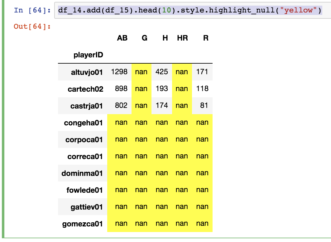
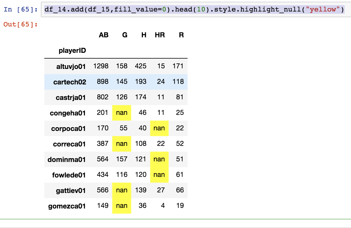
df_14.add(df_15).head(10).style.highlight_null("yellow")
style.highlight_null("yellow")这个很厉害。 没匹配上的都是空,并且没有取的列直接是空。
df_14.add(df_15,fill_value=0).head(10).style.highlight_null("yellow")
left join
被left join过来的表的index一定要唯一的,下面展开讲。
employee = pd.read_csv('data/employee.csv')
dept_sal = employee[['DEPARTMENT','BASE_SALARY']] \
            .sort_values(['DEPARTMENT','BASE_SALARY'],ascending = [True, False])
max_dept_sal = dept_sal.drop_duplicates(subset='DEPARTMENT')
max_dept_sal.head()
# 太机智了,这样就拿到最大工资了。
max_dept_sal = max_dept_sal.set_index('DEPARTMENT')
employee = employee.set_index("DEPARTMENT")
employee['MAX_DEPT_SALARY'] = max_dept_sal['BASE_SALARY']
# MAX_DEPT_SALARY 是新的,这里算是增加一列。
employee.head()
employee.query('BASE_SALARY > MAX_DEPT_SALARY')
#检验,空的,所以正确。
可以求最大值的办法,但是我觉得类似sql,感觉好low。
证明为什么left join。
employee['MAX_SALARY2'] = max_dept_sal['BASE_SALARY'].head(3)
employee.MAX_SALARY2.value_counts()
print employee.MAX_SALARY2.isnull().mean()
0.9775
缺失率那么高,当然是了left join了。
string to numeric
college = pd.read_csv('data/college.csv', index_col='INSTNM')
college.dtypes
# 把这些object都numeric化。
print college.dtypes[college.dtypes == 'object']
print college.MD_EARN_WNE_P10.value_counts().head()
# 可以拯救下。
print college.GRAD_DEBT_MDN_SUPP.value_counts().head()
print college.CITY.value_counts().head()
print college.STABBR.value_counts().head()
# 这两个没法拯救,都是string.

CITY                  object
STABBR                object
MD_EARN_WNE_P10       object
GRAD_DEBT_MDN_SUPP    object
dtype: object
PrivacySuppressed    822
38800                151
21500                 97
49200                 78
27400                 46
Name: MD_EARN_WNE_P10, dtype: int64
PrivacySuppressed    1510
9500                  514
27000                 306
25827.5               136
25000                 124
Name: GRAD_DEBT_MDN_SUPP, dtype: int64
New York       87
Chicago        78
Houston        72
Los Angeles    56
Miami          51
Name: CITY, dtype: int64
CA    773
TX    472
NY    459
FL    436
PA    394
Name: STABBR, dtype: int64

for col in ["MD_EARN_WNE_P10","GRAD_DEBT_MDN_SUPP"]:
    college[col] = pd.to_numeric(college[col],errors='coerce')
# coerce string就是np.nan.
高亮最大值
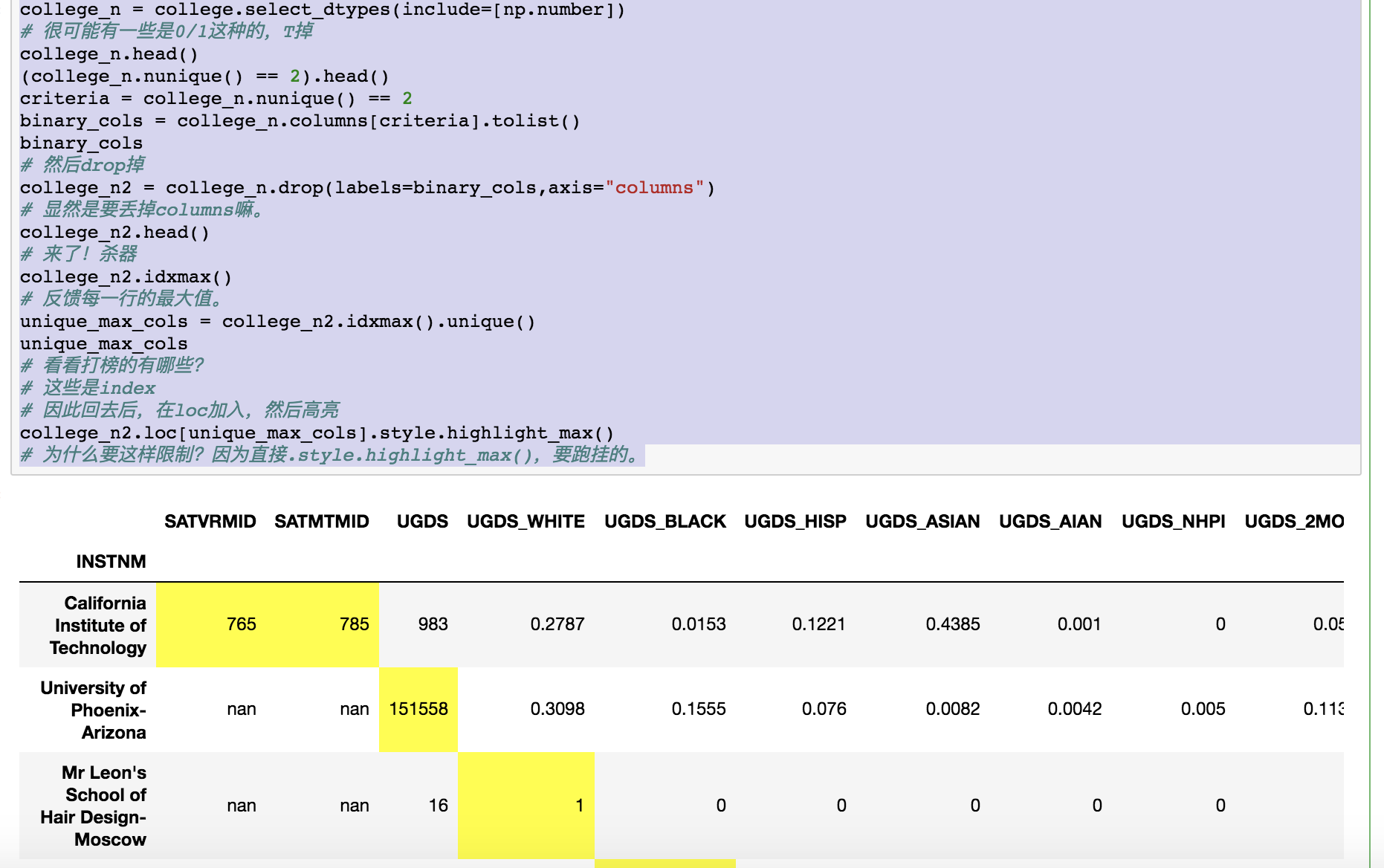
college_n = college.select_dtypes(include=[np.number])
# 很可能有一些是0/1这种的,T掉
college_n.head()
(college_n.nunique() == 2).head()
criteria = college_n.nunique() == 2
binary_cols = college_n.columns[criteria].tolist()
binary_cols
# 然后drop掉
college_n2 = college_n.drop(labels=binary_cols,axis="columns")
# 显然是要丢掉columns嘛。
college_n2.head()
# 来了!杀器
college_n2.idxmax()
# 反馈每一行的最大值。
unique_max_cols = college_n2.idxmax().unique()
unique_max_cols
# 看看打榜的有哪些?
# 这些是index
# 因此回去后,在loc加入,然后高亮
college_n2.loc[unique_max_cols].style.highlight_max()
# 为什么要这样限制?因为直接.style.highlight_max(),要跑挂的。
注意这里我们为什么可以把哪些string直接转为np.nan因为啊,它们不重要啊,我们只看最大值。
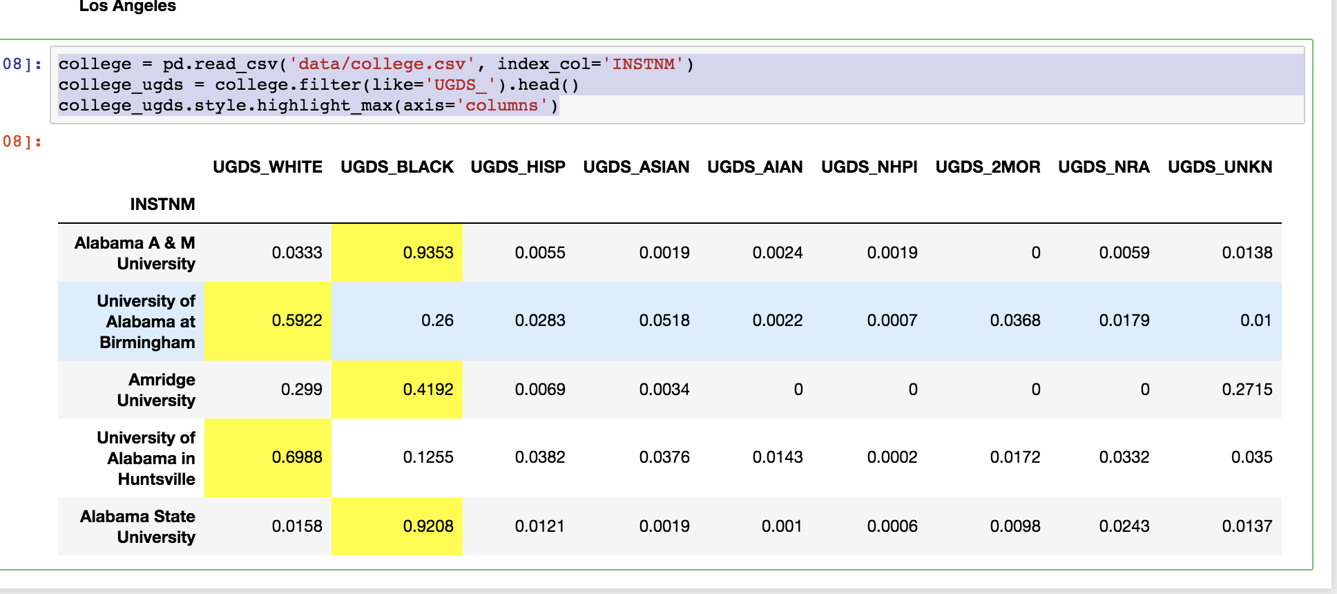
刚才是按照每列找最大值, 显然有axis的,都可以看行的, 我们就去看看那个种族歧视的样本。
college = pd.read_csv('data/college.csv', index_col='INSTNM')
college_ugds = college.filter(like='UGDS_').head()
college_ugds.style.highlight_max(axis='columns')
idxmax的另外一种写法
促行扫描。
college_n.idxmax()
# 反馈每一列最大的index
$$\arg\max_{index}(values(columns))$$
对于任意一个columns,从它的values中找到最大值,反馈这个最大值对应的index。 这个是写$\arg\max$ latex 的参考。
按照这个思路,的先有每列最大值是什么,才能去找到这个最大值处于什么位置。 总算看懂了。 这个用.max()函数知道最大值。 用eq()去定位,当然可能最大值每列中,不只一个满足条件, 这时候按照idxmax的要求,取去正常排序第一个。 那么按列cumsum()两次,那么第一个保持1的就是我们需要的。 这个时候再eq(1)就搞定了。 对于反馈的T/F矩阵,用.any(axis='columns')取出来index就好了。
college_n\
    .eq(college_n.max(axis = "columns"))\
    .cumsum(axis = "columns")\
    .cumsum(axis = "columns")\
    .eq(1)\
    .any(axis="columns")\
    .index\
    .values

array(['Alabama A & M University', 'University of Alabama at Birmingham',
       'Amridge University', ...,
       'National Personal Training Institute of Cleveland',
       'Bay Area Medical Academy - San Jose Satellite Location',
       'Excel Learning Center-San Antonio South'], dtype=object)
we can apply the
idxmaxmethod to each row of data to find the column with the largest value.axis = "columns"是answer,不是ask。
结束了,真的好累,明天第七章,早上起来看。
第七章
Hadley Wickham的想法, split $\to$ apply $\to$ combine。 这里的split就是.groupby。 这里有三种方式。
```{r echo=FALSE, message=FALSE, warning=FALSE} library(DiagrammeR) grViz( digraph dot {
graph [layout = dot]
node [shape = egg, style = filled, color = darkgreen, fontsize = 12, fontname = Helvetica, fontcolor = white, # label = ‘’]
groupby [label = ‘.groupby(…)\ntype(…)\n…GroupBy’] aggframe [label = ‘agg({…:…})’] aggseries [label = ‘agg({})’] aggseries2 [label = ‘.mean()’] frame [label = ‘pd.DataFrame’] series [label = ‘pd.Series’]
edge [ color = darkgreen, fontsize = 9, fontname = Helvetica, fontcolor = dodgerblue, label = ‘’]
groupby -> {frame series} frame -> aggframe series -> {aggseries aggseries2} }”)
flights.head() print flights.groupby(‘AIRLINE’).agg({‘ARR_DELAY’:‘mean’}).head() print type(flights.groupby(‘AIRLINE’).agg({‘ARR_DELAY’:‘mean’}).head()) # 这里的变量都要string真麻烦,不能tab智能输入。 #print flights.groupby(‘AIRLINE’).ARR_DELAY.agg(‘mean’).head() print type(flights.groupby(‘AIRLINE’).ARR_DELAY.agg(‘mean’).head()) flights.groupby(‘AIRLINE’).ARR_DELAY.mean().head()
ARR_DELAY
AIRLINE
AA 5.542661 AS -0.833333 B6 8.692593 DL 0.339691 EV 7.034580 <class ‘pandas.core.frame.DataFrame’> <class ‘pandas.core.series.Series’>
grouped = flights.groupby(‘AIRLINE’) type(grouped) pandas.core.groupby.DataFrameGroupBy
## `dplyr`的感觉
flights.groupby(‘AIRLINE’).ARR_DELAY.count() # 可以替代values_count() print flights.groupby(‘AIRLINE’).ARR_DELAY.describe() # 这个好,dplyr的感觉
count mean std min 25% 50% 75% max
AIRLINE
AA 8720.0 5.542661 43.323160 -60.0 -14.0 -5.0 9.00 858.0 AS 768.0 -0.833333 31.168354 -57.0 -14.0 -6.0 4.00 344.0 B6 540.0 8.692593 40.221718 -51.0 -13.0 -2.0 15.25 331.0 DL 10539.0 0.339691 32.299471 -57.0 -14.0 -7.0 4.00 741.0 EV 5697.0 7.034580 36.682336 -39.0 -11.0 -3.0 10.00 669.0 F9 1305.0 13.630651 53.030912 -43.0 -10.0 -1.0 17.00 839.0 HA 111.0 4.972973 37.528283 -44.0 -9.0 0.0 12.00 298.0 MQ 3314.0 6.860591 36.324657 -37.0 -13.0 -4.0 12.00 357.0 NK 1486.0 18.436070 48.727259 -39.0 -8.0 2.0 26.00 474.0 OO 6425.0 7.593463 35.331344 -44.0 -11.0 -3.0 11.00 724.0 UA 7680.0 7.765755 46.405935 -58.0 -14.0 -4.0 11.00 1185.0 US 1593.0 1.681105 27.030227 -51.0 -12.0 -4.0 7.00 431.0 VX 986.0 5.348884 33.747675 -51.0 -11.0 -3.0 8.00 236.0 WN 8310.0 6.397353 32.610666 -52.0 -11.0 -3.0 12.00 493.0
## 多个`.groupby`
flights.groupby([‘AIRLINE’,‘WEEKDAY’])[‘CANCELLED’].agg(‘sum’).head() print flights.groupby([‘AIRLINE’,‘WEEKDAY’])[‘CANCELLED’,‘DIVERTED’].agg([‘sum’,‘mean’]).head(10) # 出现mutiindex了。 # 并且这里是可以选择了列,算多个,也就是说describe都可以用,高级,比R强。
            CANCELLED           DIVERTED
                  sum      mean      sum      mean
AIRLINE WEEKDAY
AA 1 41 0.032106 6 0.004699 2 9 0.007341 2 0.001631 3 16 0.011949 2 0.001494 4 20 0.015004 5 0.003751 5 18 0.014151 1 0.000786 6 21 0.018667 9 0.008000 7 29 0.021837 1 0.000753 AS 1 0 0.000000 0 0.000000 2 0 0.000000 0 0.000000 3 0 0.000000 0 0.000000
print flights.groupby([‘AIRLINE’,‘WEEKDAY’])[‘CANCELLED’,‘DIVERTED’].agg(‘describe’).head(10)
            CANCELLED                                               \
                count      mean       std  min  25%  50%  75%  max
AIRLINE WEEKDAY
AA 1 1277.0 0.032106 0.176352 0.0 0.0 0.0 0.0 1.0
2 1226.0 0.007341 0.085399 0.0 0.0 0.0 0.0 1.0
3 1339.0 0.011949 0.108698 0.0 0.0 0.0 0.0 1.0
4 1333.0 0.015004 0.121613 0.0 0.0 0.0 0.0 1.0
5 1272.0 0.014151 0.118160 0.0 0.0 0.0 0.0 1.0
6 1125.0 0.018667 0.135405 0.0 0.0 0.0 0.0 1.0
7 1328.0 0.021837 0.146207 0.0 0.0 0.0 0.0 1.0
AS 1 118.0 0.000000 0.000000 0.0 0.0 0.0 0.0 0.0
2 106.0 0.000000 0.000000 0.0 0.0 0.0 0.0 0.0
3 115.0 0.000000 0.000000 0.0 0.0 0.0 0.0 0.0
            DIVERTED
               count      mean       std  min  25%  50%  75%  max
AIRLINE WEEKDAY
AA 1 1277.0 0.004699 0.068411 0.0 0.0 0.0 0.0 1.0
2 1226.0 0.001631 0.040373 0.0 0.0 0.0 0.0 1.0
3 1339.0 0.001494 0.038633 0.0 0.0 0.0 0.0 1.0
4 1333.0 0.003751 0.061153 0.0 0.0 0.0 0.0 1.0
5 1272.0 0.000786 0.028039 0.0 0.0 0.0 0.0 1.0
6 1125.0 0.008000 0.089124 0.0 0.0 0.0 0.0 1.0
7 1328.0 0.000753 0.027441 0.0 0.0 0.0 0.0 1.0
AS 1 118.0 0.000000 0.000000 0.0 0.0 0.0 0.0 0.0
2 106.0 0.000000 0.000000 0.0 0.0 0.0 0.0 0.0
3 115.0 0.000000 0.000000 0.0 0.0 0.0 0.0 0.0
还可以自己diy。
print flights.groupby([‘ORG_AIR’, ‘DEST_AIR’]).agg( {‘CANCELLED’:[‘sum’, ‘mean’, ‘size’, ‘count’], ‘AIR_TIME’:[‘mean’, ‘var’]} ).head()
             CANCELLED                    AIR_TIME
                   sum mean size count        mean        var
ORG_AIR DEST_AIR
ATL ABE 0 0.0 31 31 96.387097 45.778495 ABQ 0 0.0 16 16 170.500000 87.866667 ABY 0 0.0 19 19 28.578947 6.590643 ACY 0 0.0 6 6 91.333333 11.466667 AEX 0 0.0 40 40 78.725000 47.332692
注意`size`是算数量,包括空值的。
但是`count`是算非空值的。

## 去掉multiindex
flights = pd.read_csv(‘data/flights.csv’) airline_info = flights.groupby([‘AIRLINE’, ‘WEEKDAY’])
.agg({‘DIST’:[‘sum’,‘mean’], ‘ARR_DELAY’:[‘max’,‘min’]})
.astype(int) # .info() # 为了减少内存,用int,不用float。 airline_info.head()
            ARR_DELAY         DIST
                  max min      sum  mean
AIRLINE WEEKDAY
AA 1 551 -60 1455386 1139 2 725 -52 1358256 1107 3 473 -45 1496665 1117 4 349 -46 1452394 1089 5 732 -41 1427749 1122
print airline_info.columns print airline_info.columns.get_level_values(0) print airline_info.columns.get_level_values(1)
MultiIndex(levels=[[u’ARR_DELAY’, u’DIST’], [u’max’, u’mean’, u’min’, u’sum’]], labels=[[0, 0, 1, 1], [0, 2, 3, 1]]) Index([u’ARR_DELAY’, u’ARR_DELAY’, u’DIST’, u’DIST’], dtype=‘object’) Index([u’max’, u’min’, u’sum’, u’mean’], dtype=‘object’)
这样挺好,我有idea了,之后合并就好。
airline_info.columns.get_level_values(0) + ‘_’ + airline_info.columns.get_level_values(1) Index([u’ARR_DELAY_max’, u’ARR_DELAY_min’, u’DIST_sum’, u’DIST_mean’], dtype=‘object’)
print airline_info.head() ARR_DELAY_max ARR_DELAY_min DIST_sum DIST_mean AIRLINE WEEKDAY
AA 1 551 -60 1455386 1139 2 725 -52 1358256 1107 3 473 -45 1496665 1117 4 349 -46 1452394 1089 5 732 -41 1427749 1122
print airline_info.reset_index().head() AIRLINE WEEKDAY ARR_DELAY_max ARR_DELAY_min DIST_sum DIST_mean 0 AA 1 551 -60 1455386 1139 1 AA 2 725 -52 1358256 1107 2 AA 3 473 -45 1496665 1117 3 AA 4 349 -46 1452394 1089 4 AA 5 732 -41 1427749 1122
这样未免有点太复杂,实际上有简便的方法。
print flights.groupby([‘AIRLINE’], as_index=False)[‘DIST’].agg(‘mean’)
.round(0)
.head() AIRLINE DIST 0 AA 1114.0 1 AS 1066.0 2 B6 1772.0 3 DL 866.0 4 EV 460.0
`pd.DataFrame.groupby?`中,
as_index : boolean, default True For aggregated output, return object with group labels as the index. Only relevant for DataFrame input. as_index=False is effectively “SQL-style” grouped output
`as_index`表示是否把grouping columns变成index。
`sort`表示grouping columns是否sort。

## 自己设计汇总函数
print college.groupby([‘STABBR’, ‘RELAFFIL’])
[‘UGDS’, ‘SATVRMID’, ‘SATMTMID’]
.agg([max_deviation,‘mean’,‘std’]).round(1).head()
                     UGDS                      SATVRMID               \
            Max Deviation    mean     std Max Deviation   mean   std
STABBR RELAFFIL
AK 0 2.1 3508.9 4539.5 NaN NaN NaN
1 1.1 123.3 132.9 NaN 555.0 NaN
AL 0 5.2 3248.8 5102.4 1.6 514.9 56.5
1 2.4 979.7 870.8 1.5 498.0 53.0
AR 0 5.8 1793.7 3401.6 1.9 481.1 37.9
                 SATMTMID
            Max Deviation   mean   std
STABBR RELAFFIL
AK 0 NaN NaN NaN
1 NaN 503.0 NaN
AL 0 1.7 515.8 56.7
1 1.4 485.6 61.4
AR 0 2.0 503.6 39.0
## nest function
def pct_between_1_3k(s): return s.between(1000, 3000).mean() print college.groupby([‘STABBR’, ‘RELAFFIL’])[‘UGDS’]
.agg(pct_between_1_3k).head(9) STABBR RELAFFIL AK 0 0.142857 1 0.000000 AL 0 0.236111 1 0.333333 AR 0 0.279412 1 0.111111 AS 0 1.000000 AZ 0 0.096774 1 0.000000 Name: UGDS, dtype: float64
def pct_between(s, low, high): return s.between(low, high).mean() print college.groupby([‘STABBR’, ‘RELAFFIL’])[‘UGDS’]
.agg(pct_between, 1000, 10000).head(9) STABBR RELAFFIL AK 0 0.428571 1 0.000000 AL 0 0.458333 1 0.375000 AR 0 0.397059 1 0.166667 AS 0 1.000000 AZ 0 0.233871 1 0.111111 Name: UGDS, dtype: float64
如果agg的函数有其他参数,必须先设定好了再弄。
def make_agg_func(func, name, *args,**kwargs): def wrapper(x): return func(x, *args, **kwargs) wrapper.__name__ = name return wrapper my_agg1 = make_agg_func(pct_between, ‘pct_1_3k’, low=1000, high=3000) my_agg2 = make_agg_func(pct_between, ‘pct_10_30k’, 10000, 30000) print college.groupby([‘STABBR’, ‘RELAFFIL’])[‘UGDS’]
.agg([‘mean’, my_agg1, my_agg2]).head()
mean pct_1_3k pct_10_30k
STABBR RELAFFIL
AK 0 3508.857143 0.142857 0.142857 1 123.333333 0.000000 0.000000 AL 0 3248.774648 0.236111 0.083333 1 979.722222 0.333333 0.000000 AR 0 1793.691176 0.279412 0.014706
## dive in 每组的情况
college = pd.read_csv(‘data/college.csv’) grouped = college.groupby([‘STABBR’, ‘RELAFFIL’]) type(grouped) pandas.core.groupby.DataFrameGroupBy
dir?
for a class object: its attributes, and recursively the attributes
of its bases.
包括变量等等attr
我们知道__name__这些不好,就T掉,
用if not
dir(grouped) print pd.Series([attr for attr in dir(grouped) if not attr.startswith(’_’)]).head()
0 CITY 1 CURROPER 2 DISTANCEONLY 3 GRAD_DEBT_MDN_SUPP 4 HBCU dtype: object
print grouped.ngroups # 查看多少个组 type(grouped.groups) # dict style grouped.groups.keys()[:6] print grouped.get_group((‘FL’, 1)).iloc[:,:3].head() # 可以具体看那一期
112 INSTNM CITY STABBR 712 The Baptist College of Florida Graceville FL 713 Barry University Miami FL 714 Gooding Institute of Nurse Anesthesia Panama City FL 715 Bethune-Cookman University Daytona Beach FL 724 Johnson University Florida Kissimmee FL
from IPython.display import display for name, group in grouped: print(name) display(group.head(3)) # name就是group的tuple, # group就是具体的nest frame # display就是展示,真好。
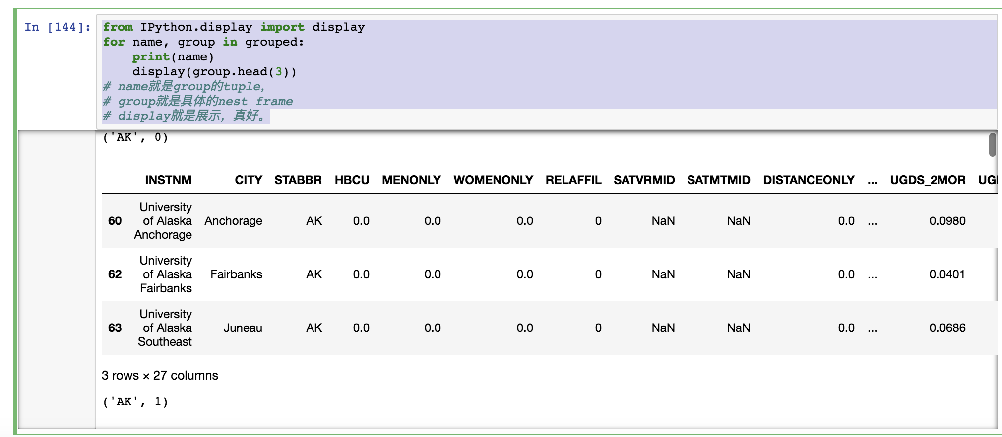
每一组都展示了,我觉得很不错。
直接head也可以
grouped.head(2)
这样就全部展示了,每个group的前两排
print grouped.head(2).head(10).iloc[:,:3]
INSTNM CITY STABBR
0 Alabama A & M University Normal AL 1 University of Alabama at Birmingham Birmingham AL 2 Amridge University Montgomery AL 10 Birmingham Southern College Birmingham AL 43 Prince Institute-Southeast Elmhurst IL 60 University of Alaska Anchorage Anchorage AK 61 Alaska Bible College Palmer AK 62 University of Alaska Fairbanks Fairbanks AK 64 Alaska Pacific University Anchorage AK 68 Everest College-Phoenix Phoenix AZ
根据`head(2)`的启发,我们是否可以特定的拿?可以的,用`nth`。
print grouped.nth([1, -1]).head(8).iloc[:,:3] CITY CURROPER DISTANCEONLY STABBR RELAFFIL
AK 0 Fairbanks 1 0.0 0 Barrow 1 0.0 1 Anchorage 1 0.0 1 Soldotna 1 0.0 AL 0 Birmingham 1 0.0 0 Dothan 1 0.0 1 Birmingham 1 0.0 1 Huntsville 1 NaN
你看是不是每组的首行和尾行。

## minority majority
相当于每个groupby后反馈一个汇总值。
def check_minority(df, threshold): minority_pct = 1 - df[‘UGDS_WHITE’] total_minority = (df[‘UGDS’] * minority_pct).sum() total_ugds = df[‘UGDS’].sum() total_minority_pct = total_minority / total_ugds return total_minority_pct > threshold # 反馈那些大于threshold的非白人群占比的一排,因为有很多组,因此反馈59行嘛? # 不是而是只要总体满足这个要求,那么每个被汇总量也会被反馈,因此叫做minority majority # 因此实际上只是grouping cloumns被筛选,里面的娃都是一刀切,T or F,all in。 print college_filtered = grouped.filter(check_minority, threshold=.5) college_filtered.iloc[:,:1].head() print college.shape print college_filtered.shape print college_filtered[‘STABBR’].nunique() # The goal is to keep all the rows from the states, as a whole # 注意as a whole,全部!!!
以上是反馈筛选后的group,和每个group里面未减少的rows。

## 保留group、组内筛选

现在进行的是,group全部保留,但是在每个group里面筛选。
weight_loss = pd.read_csv(‘data/weight_loss.csv’) print weight_loss.head(10)
Name Month Week Weight 0 Bob Jan Week 1 291 1 Amy Jan Week 1 197 2 Bob Jan Week 2 288 3 Amy Jan Week 2 189 4 Bob Jan Week 3 283 5 Amy Jan Week 3 189 6 Bob Jan Week 4 283 7 Amy Jan Week 4 190 8 Bob Feb Week 1 283 9 Amy Feb Week 1 190
weight_loss.query(‘Month == “Jan”’) def find_perc_loss(s): return (s-s.iloc[0])/s.iloc[0] bob_jan = weight_loss.query(‘Name==“Bob” and Month == “Jan”’) bob_jan find_perc_loss(bob_jan.Weight) # 这个时候是groupby和transform的合作了。 weight_loss.groupby([‘Name’,‘Month’]).Weight.transform(find_perc_loss)
.head() weight_loss[‘Perc Weight Loss’]=weight_loss.groupby([‘Name’,‘Month’]).Weight.transform(find_perc_loss).round(3) # 那么看一下, weight_loss.query(‘Name==“Bob” and Month in [“Jan”, “Feb”]’) week4 = weight_loss.query(‘Week == “Week 4”’) print week4
Name Month Week Weight Perc Weight Loss 6 Bob Jan Week 4 283 -0.027 7 Amy Jan Week 4 190 -0.036 14 Bob Feb Week 4 268 -0.053 15 Amy Feb Week 4 173 -0.089 22 Bob Mar Week 4 261 -0.026 23 Amy Mar Week 4 170 -0.017 30 Bob Apr Week 4 250 -0.042 31 Amy Apr Week 4 161 -0.053
然后对week4,进行spread分析了。
winner = week4.pivot(index = ‘Month’,columns = ‘Name’,values = ‘Perc Weight Loss’) winner # 加一下winner # 类似于if-then条件 winner[‘Winner’] = np.where( winner[‘Amy’] < winner[‘Bob’], ‘Amy’, ‘Bob’ ) winner.style.highlight_min(axis=‘columns’) # 每行产生一个值,形成一列,所以axis=‘columns’ # 但是Month的时间顺序改变了。
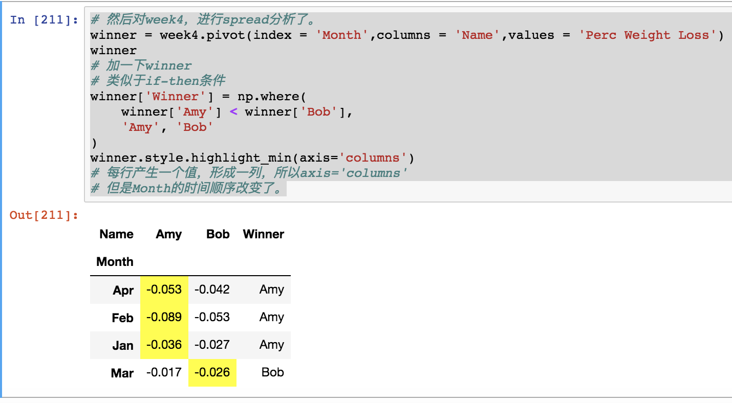
我们知道week4是对的,用它的排序
print week4.Month.unique() winner.index = pd.Categorical(winner.index, categories = week4.Month.unique(), ordered=True) print winner # 没有用 # 因为index是tuple,忘了?
[‘Jan’ ‘Feb’ ‘Mar’ ‘Apr’] Name Amy Bob Winner Apr -0.053 -0.042 Amy Feb -0.089 -0.053 Amy Jan -0.036 -0.027 Amy Mar -0.017 -0.026 Bob
week4a = week4.copy() month_chron = week4a[‘Month’].unique() month_chron week4a[‘Month’] = pd.Categorical(week4a[‘Month’], categories=month_chron, ordered=True) print week4a.pivot(index=‘Month’, columns=‘Name’, values=‘Perc Weight Loss’) Name Amy Bob Month
Jan -0.036 -0.027 Feb -0.089 -0.053 Mar -0.017 -0.026 Apr -0.053 -0.042
## `groupby`和`apply`函数

`groupby` $\to$
`agg`, `filter`, `transform`, 和 `apply`。

+ `agg`: scalar value
+ `filter`: boolean
+ `transform`: Series,row数量不变
+ `apply`: 以上三都可以,连DataFrame都可以。
college = pd.read_csv(‘data/college.csv’) subset = [‘UGDS’, ‘SATMTMID’, ‘SATVRMID’] college2 = college.dropna(subset=subset) print college.shape print college2.shape college2.head()[[‘UGDS’, ‘SATMTMID’, ‘SATVRMID’,‘STABBR’]] def weighted_math_average(df): weighted_math = df.SATVRMID * df.UGDS return weighted_math.sum()/df.UGDS.sum() print college2.groupby(‘STABBR’).apply(weighted_math_average).head() print college2[[‘UGDS’, ‘SATMTMID’, ‘SATVRMID’,‘STABBR’]].groupby(‘STABBR’).agg(weighted_math_average).head().iloc[:,:3] # agg不好,不能自定义具体那一列来计算 # transform是反馈一个series而非一个值。
(7535, 27) (1184, 27) STABBR AK 555.000000 AL 533.383387 AR 504.876157 AZ 557.303350 CA 539.316605 dtype: float64 UGDS SATMTMID SATVRMID STABBR
AK 555.000000 555.000000 555.000000 AL 533.383387 533.383387 533.383387 AR 504.876157 504.876157 504.876157 AZ 557.303350 557.303350 557.303350 CA 539.316605 539.316605 539.316605
`agg`中`SATMTMID`和`SATVRMID`都反馈了我们想要的。

> Directly replacing `apply` with `agg` does not work as agg returns a value for each of its aggregating columns.
college2.groupby(‘STABBR’)[‘SATMTMID’]
.agg(weighted_math_average) KeyError: ‘UGDS’
因此做这种处理时,存在多个col时,应该用`apply`而非`agg`。

再深化一下,为什么apply更好,是因为 还可以自定义反馈多少的列。
OrderedDict在这里是关键。
确实反馈一条series,每个group一行。
from collections import OrderedDict def weighted_average(df): data = OrderedDict() weight_m = df.UGDS * df.SATMTMID weight_v = df.UGDS * df.SATVRMID wm_avg = weight_m.sum() / df[‘UGDS’].sum() wv_avg = weight_v.sum() / df[‘UGDS’].sum()
data['weighted_math_avg'] = wm_avg
data['weighted_verbal_avg'] = wv_avg
data['math_avg'] = df['SATMTMID'].mean()
data['verbal_avg'] = df['SATVRMID'].mean()
data['count'] = len(df)
return pd.Series(data, dtype='int')
print college2.groupby(‘STABBR’).apply(weighted_average).head(10)
weighted_math_avg weighted_verbal_avg math_avg verbal_avg count
STABBR
AK 503 555 503 555 1 AL 536 533 504 508 21 AR 529 504 515 491 16 AZ 569 557 536 538 6 CA 564 539 562 549 72 CO 553 547 540 537 14 CT 545 533 522 517 14 DC 621 623 588 589 6 DE 569 553 495 486 3 FL 565 565 521 529 38
其实还可以是反馈frame,这体现在multiindex嘛,因为是frame啊,除了columns还有index。
from scipy.stats import gmean, hmean def calculate_means(df): df_means = pd.DataFrame(index=[‘Arithmetic’, ‘Weighted’, ‘Geometric’, ‘Harmonic’]) cols = [‘SATMTMID’, ‘SATVRMID’] for col in cols: arithmetic = df[col].mean() weighted = np.average(df[col], weights=df[‘UGDS’]) geometric = gmean(df[col]) harmonic = hmean(df[col]) df_means[col] = [arithmetic, weighted, geometric, harmonic] df_means[‘count’] = len(df) return df_means.astype(int) print college2.groupby(‘STABBR’).apply(calculate_means).head(12)
SATMTMID SATVRMID count
STABBR
AK Arithmetic 503 555 1 Weighted 503 555 1 Geometric 503 555 1 Harmonic 503 555 1 AL Arithmetic 504 508 21 Weighted 536 533 21 Geometric 500 505 21 Harmonic 497 502 21 AR Arithmetic 515 491 16 Weighted 529 504 16 Geometric 514 489 16 Harmonic 513 487 16
## 变量切bin
flights = pd.read_csv(‘data/flights.csv’) flights.head() bins = [-np.inf, 200, 500, 1000, 2000, np.inf] cuts = pd.cut(flights[‘DIST’], bins=bins) cuts.head()
0 (500.0, 1000.0] 1 (1000.0, 2000.0] 2 (500.0, 1000.0] 3 (1000.0, 2000.0] 4 (1000.0, 2000.0] Name: DIST, dtype: category Categories (5, interval[float64]): [(-inf, 200.0] < (200.0, 500.0] < (500.0, 1000.0] < (1000.0, 2000.0] < (2000.0, inf]]
`Categories`都打好顺序的标签了。
cuts.value_counts() flights.groupby(cuts)[‘AIRLINE’].value_counts(normalize=True)
.round(3).head(15)
DIST AIRLINE (-inf, 200.0] OO 0.326 EV 0.289 MQ 0.211 DL 0.086 AA 0.052 UA 0.027 WN 0.009 (200.0, 500.0] WN 0.194 DL 0.189 OO 0.159 EV 0.156 MQ 0.100 AA 0.071 UA 0.062 VX 0.028 Name: AIRLINE, dtype: float64
flights.groupby(cuts)[‘AIR_TIME’].quantile(q=[.25, .5, .75])
.div(60).round(2)
DIST
(-inf, 200.0] 0.25 0.43 0.50 0.50 0.75 0.57 (200.0, 500.0] 0.25 0.77 0.50 0.92 0.75 1.05 (500.0, 1000.0] 0.25 1.43 0.50 1.65 0.75 1.92 (1000.0, 2000.0] 0.25 2.50 0.50 2.93 0.75 3.40 (2000.0, inf] 0.25 4.30 0.50 4.70 0.75 5.03 Name: AIR_TIME, dtype: float64
不好看不喜欢,用`unstack`。
print flights.groupby(cuts)[‘AIR_TIME’].quantile(q=[.25, .5, .75])
.div(60).round(2)
.unstack()
0.25 0.50 0.75
DIST
(-inf, 200.0] 0.43 0.50 0.57 (200.0, 500.0] 0.77 0.92 1.05 (500.0, 1000.0] 1.43 1.65 1.92 (1000.0, 2000.0] 2.50 2.93 3.40 (2000.0, inf] 4.30 4.70 5.03
labels=[‘Under an Hour’, ‘1 Hour’, ‘1-2 Hours’, ‘2-4 Hours’, ‘4+ Hours’] # 需要改下bin的label,太难看了。 cuts2 = pd.cut(flights[‘DIST’], bins=bins, labels=labels) flights.groupby(cuts2)[‘AIRLINE’].value_counts(normalize=True)
.round(3)
.unstack()
.style.highlight_max(axis=1)
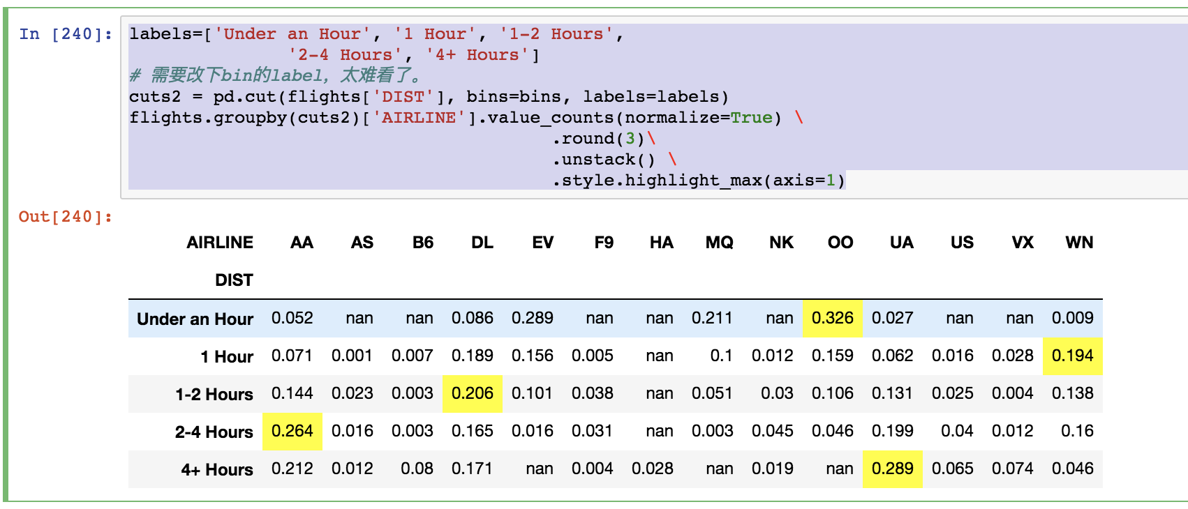
这里,`.highlight_max(axis=1)`表示每行反馈一个,可以组成一列。
## `sorted`函数
flights = pd.read_csv(‘data/flights.csv’) flights_ct = flights.groupby([‘ORG_AIR’, ‘DEST_AIR’]).size() flights_ct.head() # 我感觉,应该是sorted函数剔除重复项目 flights_ct.loc[[(‘ATL’, ‘IAH’), (‘IAH’, ‘ATL’)]]
ORG_AIR DEST_AIR ATL IAH 121 IAH ATL 148 dtype: int64
flights_sort = flights[[‘ORG_AIR’, ‘DEST_AIR’]]
.apply(sorted, axis=1) flights_sort.head() # 我感觉sorted,可以让A->B 和 A<-B合并
有`sorted`函数跑的太慢了。
ORG_AIR DEST_AIR 0 LAX SLC 1 DEN IAD 2 DFW VPS 3 DCA DFW 4 LAX MCI
rename_dict = {‘ORG_AIR’:‘AIR1’, ‘DEST_AIR’:‘AIR2’} flights_sort = flights_sort.rename(columns=rename_dict) flights_ct2 = flights_sort.groupby([‘AIR1’, ‘AIR2’]).size() print flights_ct2.head() print flights_ct2.loc[(‘ATL’, ‘IAH’)]
AIR1 AIR2 ABE ATL 31 ORD 24 ABI DFW 74 ABQ ATL 16 DEN 46 dtype: int64 269
这个`269`说明问题了,真的合并了。
flights_ct2.loc[(‘IAH’, ‘ATL’)] IndexingError: Too many indexers
报错了。

这里推荐使用`np.sort`。
data_sorted = np.sort(flights[[‘ORG_AIR’, ‘DEST_AIR’]]) data_sorted[:10] flights_sort2 = pd.DataFrame(data_sorted, columns = [‘AIR1’,‘AIR2’]) fs_orig = flights_sort.rename(columns={‘ORG_AIR’:‘AIR1’, ‘DEST_AIR’:‘AIR2’}) print flights_sort2.equals(fs_orig) True
一致的。
%%timeit flights_sort = flights[[‘ORG_AIR’, ‘DEST_AIR’]]
.apply(sorted, axis=1) 1 loop, best of 3: 10.6 s per loop
太慢了,别瞎跑。
%%timeit data_sorted = np.sort(flights[[‘ORG_AIR’, ‘DEST_AIR’]]) flights_sort2 = pd.DataFrame(data_sorted, columns=[‘AIR1’, ‘AIR2’]) 100 loops, best of 3: 11 ms per loop
这就是`numpy`的力量。

## 连续n次准时metric求解
s = pd.Series([0, 1, 1, 0, 1, 1, 1, 0]) print s # 假设这是一架飞机的飞行记录,1表示准时,0表示不准时, # 理论上,这里发生了2次连续准时,3次准时,表达出来就好了。 s1 = s.cumsum() s1 print s.mul(s1).diff().where(lambda x: x < 0).ffill().add(s1,fill_value=0)
0 0 1 1 2 1 3 0 4 1 5 1 6 1 7 0 dtype: int64 0 0.0 1 1.0 2 2.0 3 0.0 4 1.0 5 2.0 6 3.0 7 0.0 dtype: float64
但是我现在对这个为什么要这么函数求解不太懂!!!
推出来!!!
然后开始跑模型。
pd.Series.lt?
flights = pd.read_csv(‘data/flights.csv’) flights[‘ON_TIME’] = flights[‘ARR_DELAY’].lt(15).astype(int) flights[[‘AIRLINE’, ‘ORG_AIR’, ‘ON_TIME’]].head(10) flights[[‘AIRLINE’, ‘ORG_AIR’, ‘ON_TIME’]].shape def max_streak(s): s1 = s.cumsum() return s.mul(s1).diff().where(lambda x: x < 0)
.ffill().add(s1, fill_value=0).max() print flights.sort_values([‘MONTH’, ‘DAY’, ‘SCHED_DEP’])
.groupby([‘AIRLINE’, ‘ORG_AIR’])[‘ON_TIME’]
.agg([‘mean’, ‘size’, max_streak]).round(2).head()
mean size max_streak
AIRLINE ORG_AIR
AA ATL 0.82 233 15 DEN 0.74 219 17 DFW 0.78 4006 64 IAH 0.80 196 24 LAS 0.79 374 29
streak = s.mul(s1).diff().where(lambda x: x < 0).ffill().add(s1,fill_value=0) print streak print streak.idxmax() # 就是最长的这次streak最后一次在哪个index。 print streak.max() # 就是最长的这次streak多长 print streak.idxmax() - streak.max() + 1 # 就是最长的这次streak哪个index开始的。
def max_delay_streak(df): df = df.reset_index(drop=True) s = 1 - df[‘ON_TIME’] s1 = s.cumsum() streak = s.mul(s1).diff().where(lambda x: x < 0)
.ffill().add(s1, fill_value=0) last_idx = streak.idxmax() first_idx = last_idx - streak.max() + 1 df_return = df.loc[[first_idx, last_idx], [‘MONTH’, ‘DAY’]] df_return[‘streak’] = streak.max() df_return.index = [‘first’, ’last’] df_return.index.name=‘type’ return df_return print flights.sort_values([‘MONTH’, ‘DAY’, ‘SCHED_DEP’])
.groupby([‘AIRLINE’, ‘ORG_AIR’])
.apply(max_delay_streak)
.sort_values(‘streak’, ascending=False).head(10)
MONTH DAY streak
AIRLINE ORG_AIR type
AA DFW first 2.0 26.0 38.0 last 3.0 1.0 38.0 MQ ORD last 1.0 12.0 28.0 first 1.0 6.0 28.0 DFW last 2.0 26.0 25.0 first 2.0 21.0 25.0 NK ORD first 6.0 7.0 15.0 last 6.0 18.0 15.0 DL ATL last 12.0 24.0 14.0 first 12.0 23.0 14.0
2月26日到3月1日,38次delay,真尴尬。

# 第八章

## stack查看index的情况
state_fruit = pd.read_csv(‘data/state_fruit.csv’, index_col=0) state_fruit print state_fruit.stack() # stack 就是把所有columns放到index这边 # 你看index上没有命名。 state_fruit_tidy = state_fruit.stack().reset_index() print state_fruit_tidy # 需要改一下columns的命名, # 注意这里他们都是columns了,不是index了 # reset_index有毒。 state_fruit_tidy.columns = [‘state’, ‘fruit’, ‘weight’] print state_fruit_tidy
Texas Apple 12 Orange 10 Banana 40 Arizona Apple 9 Orange 7 Banana 12 Florida Apple 0 Orange 14 Banana 190 dtype: int64 level_0 level_1 0 0 Texas Apple 12 1 Texas Orange 10 2 Texas Banana 40 3 Arizona Apple 9 4 Arizona Orange 7 5 Arizona Banana 12 6 Florida Apple 0 7 Florida Orange 14 8 Florida Banana 190 state fruit weight 0 Texas Apple 12 1 Texas Orange 10 2 Texas Banana 40 3 Arizona Apple 9 4 Arizona Orange 7 5 Arizona Banana 12 6 Florida Apple 0 7 Florida Orange 14 8 Florida Banana 190
state_fruit.stack()
.rename_axis([‘state’, ‘fruit’])
.reset_index(name=‘weight’)
state fruit weight
0 Texas Apple 12 1 Texas Orange 10 2 Texas Banana 40 3 Arizona Apple 9 4 Arizona Orange 7 5 Arizona Banana 12 6 Florida Apple 0 7 Florida Orange 14 8 Florida Banana 190
`.rename_axis`给index命名。
`.reset_index`有`name`可以设置变量,columns的命名。
当然`.reset_index`了,index就变成变量了。
state_fruit2 = pd.read_csv(‘data/state_fruit2.csv’) state_fruit2 print state_fruit2.stack() print state_fruit2.set_index(‘State’).stack()
当数据表没有index的时候,要想方设法设立一个index才行。
`set_index('State')`。
0 State Texas Apple 12 Orange 10 Banana 40 1 State Arizona Apple 9 Orange 7 Banana 12 2 State Florida Apple 0 Orange 14 Banana 190 dtype: object State
Texas Apple 12 Orange 10 Banana 40 Arizona Apple 9 Orange 7 Banana 12 Florida Apple 0 Orange 14 Banana 190 dtype: int64
## `melt`函数

等于R中`dplyr`中的`gather`。
其实注意了,gather后本来,index会变,悄悄的变,然后替换上默认的index。
state_fruit2 = pd.read_csv(‘data/state_fruit2.csv’) print state_fruit2.set_index(‘State’).stack().reset_index() print state_fruit2.melt(id_vars=[‘State’]) print state_fruit2.melt(id_vars=[‘State’],value_vars=[‘Apple’,‘Orange’,‘Banana’]) print state_fruit2.melt(id_vars=[‘State’], value_vars=[‘Apple’,‘Orange’,‘Banana’], var_name = ‘Fruit’, value_name = ‘Weight’) # 全部几乎一样,是否感觉pandas就是啰嗦?
State level_1 0
0 Texas Apple 12 1 Texas Orange 10 2 Texas Banana 40 3 Arizona Apple 9 4 Arizona Orange 7 5 Arizona Banana 12 6 Florida Apple 0 7 Florida Orange 14 8 Florida Banana 190 State variable value 0 Texas Apple 12 1 Arizona Apple 9 2 Florida Apple 0 3 Texas Orange 10 4 Arizona Orange 7 5 Florida Orange 14 6 Texas Banana 40 7 Arizona Banana 12 8 Florida Banana 190 State variable value 0 Texas Apple 12 1 Arizona Apple 9 2 Florida Apple 0 3 Texas Orange 10 4 Arizona Orange 7 5 Florida Orange 14 6 Texas Banana 40 7 Arizona Banana 12 8 Florida Banana 190 State Fruit Weight 0 Texas Apple 12 1 Arizona Apple 9 2 Florida Apple 0 3 Texas Orange 10 4 Arizona Orange 7 5 Florida Orange 14 6 Texas Banana 40 7 Arizona Banana 12 8 Florida Banana 190
## 一次性完成两个gather运算

好累,ddl就是明天了,不能晚了,赶紧刷完了。

`DataFrame.rename`
这个函数是直接作用于frame,
并且对象直接是index和columns。
s = pd.Series([1, 2, 3]) s 0 1 1 2 2 3 dtype: int64 s.rename(“my_name”) # scalar, changes Series.name 0 1 1 2 2 3 Name: my_name, dtype: int64 s.rename(lambda x: x ** 2) # function, changes labels 0 1 1 2 4 3 dtype: int64 s.rename({1: 3, 2: 5}) # mapping, changes labels 0 1 3 2 5 3 dtype: int64
def change_col_name(col_name): col_name = col_name.replace(’_name’, ‘’) if ‘facebook’ in col_name: fb_idx = col_name.find(‘facebook’) col_name = col_name[:5] + col_name[fb_idx - 1:]\
- col_name[5:fb_idx-1] return col_name # 解构这个函数 # 这个函数暂时解构不出来,因为他不确定它面向对象的格式, # 这个之后再说吧。
movie = pd.read_csv(‘data/movie.csv’) actor = movie[[‘movie_title’, ‘actor_1_name’, ‘actor_2_name’, ‘actor_3_name’, ‘actor_1_facebook_likes’, ‘actor_2_facebook_likes’, ‘actor_3_facebook_likes’]] actor.head() # 函数开始应用。 actor2 = actor.rename(columns=change_col_name) print actor2.head() stubs = [‘actor’, ‘actor_facebook_likes’] # 类似于gather里面的被gather的列表 # i是k不动的对象, # j是key, # stubs其实是value actor2_tidy = pd.wide_to_long(actor2, stubnames=stubs, i=[‘movie_title’], j=‘actor_num’, sep=’_’) print actor2_tidy.head()
movie_title actor_1 \
0 Avatar CCH Pounder
1 Pirates of the Caribbean: At World’s End Johnny Depp
2 Spectre Christoph Waltz
3 The Dark Knight Rises Tom Hardy
4 Star Wars: Episode VII - The Force Awakens Doug Walker
actor_2 actor_3 actor_facebook_likes_1 \
0 Joel David Moore Wes Studi 1000.0
1 Orlando Bloom Jack Davenport 40000.0
2 Rory Kinnear Stephanie Sigman 11000.0
3 Christian Bale Joseph Gordon-Levitt 27000.0
4 Rob Walker NaN 131.0
actor_facebook_likes_2 actor_facebook_likes_3
0 936.0 855.0
1 5000.0 1000.0
2 393.0 161.0
3 23000.0 23000.0
4 12.0 NaN
actor
movie_title actor_num
Avatar 1 CCH Pounder
Pirates of the Caribbean: At World’s End 1 Johnny Depp
Spectre 1 Christoph Waltz
The Dark Knight Rises 1 Tom Hardy
Star Wars: Episode VII - The Force Awakens 1 Doug Walker
actor_facebook_likes
movie_title actor_num
Avatar 1 1000.0
Pirates of the Caribbean: At World’s End 1 40000.0
Spectre 1 11000.0
The Dark Knight Rises 1 27000.0
Star Wars: Episode VII - The Force Awakens 1 131.0
`pd.wide_to_long`
必须得好好研究一下。
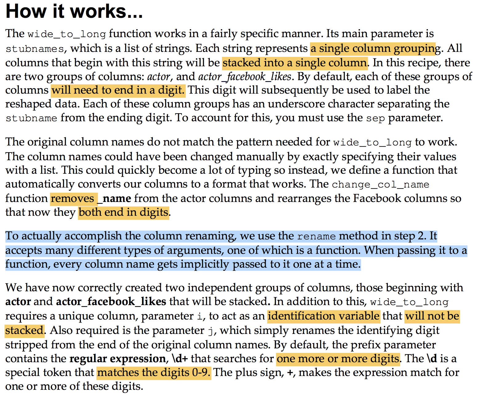
加油啊!!!
ddl!
## `unstack`和`pivot` spread的兄弟
类似于R的`dplyr`的`spread`函数
pd.read_csv?
usecols : array-like or callable, default None
Return a subset of the columns. If array-like, all elements must either
be positional (i.e. integer indices into the document columns) or strings
that correspond to column names provided either by the user in names or
inferred from the document header row(s). For example, a valid array-like
usecols parameter would be [0, 1, 2] or [‘foo’, ‘bar’, ‘baz’].
If callable, the callable function will be evaluated against the column
names, returning names where the callable function evaluates to True. An
example of a valid callable argument would be lambda x: x.upper() in # ['AAA', 'BBB', 'DDD']. Using this parameter results in much faster
parsing time and lower memory usage.
非常好用,类似于filter的%in%条件,还可以多个并行
usecol_func = lambda x: ‘UGDS_’ in x or x == ‘INSTNM’ college = pd.read_csv(‘data/college.csv’, index_col=‘INSTNM’, usecols=usecol_func) college.stack().unstack()
.head() # dropna=False 这个参数可以注意加,因为dropna默认是True college2 = pd.read_csv(‘data/college.csv’, usecols=usecol_func) print college2.melt(id_vars=‘INSTNM’, var_name = ‘Race’, value_name = ‘Percentage’)
.head() # 更加灵活,跟index没关系。 print college2.melt(id_vars=‘INSTNM’, var_name = ‘Race’, value_name = ‘Percentage’)
.pivot(index = ‘INSTNM’, columns = ‘Race’, values = ‘Percentage’)
.head().iloc[:,:1]
INSTNM Race Percentage
0 Alabama A & M University UGDS_WHITE 0.0333 1 University of Alabama at Birmingham UGDS_WHITE 0.5922 2 Amridge University UGDS_WHITE 0.2990 3 University of Alabama in Huntsville UGDS_WHITE 0.6988 4 Alabama State University UGDS_WHITE 0.0158 Race UGDS_2MOR INSTNM
A & W Healthcare Educators 0.0000 A T Still University of Health Sciences NaN ABC Beauty Academy 0.0000 ABC Beauty College Inc 0.0000 AI Miami International University of Art and De… 0.0018
保证index和columns的顺序。
print college2.melt(id_vars=‘INSTNM’, var_name = ‘Race’, value_name = ‘Percentage’)
.pivot(index = ‘INSTNM’, columns = ‘Race’, values = ‘Percentage’)
.loc[college2[‘INSTNM’], college2.columns[1:]]
.reset_index()
.head().iloc[:,:3]
INSTNM UGDS_WHITE UGDS_BLACK
0 Alabama A & M University 0.0333 0.9353 1 University of Alabama at Birmingham 0.5922 0.2600 2 Amridge University 0.2990 0.4192 3 University of Alabama in Huntsville 0.6988 0.1255 4 Alabama State University 0.0158 0.9208
>>> college2.equals(college2_replication)
True
## `unstack`特定一个变量,增加灵活性
employee = pd.read_csv(‘data/employee.csv’) employee.groupby(‘RACE’)[‘BASE_SALARY’].mean().astype(int) employee.groupby([‘RACE’, ‘GENDER’])[‘BASE_SALARY’]
.mean().astype(int)
.unstack(‘GENDER’) print employee.groupby([‘RACE’, ‘GENDER’])[‘BASE_SALARY’]
.agg([‘mean’, ‘max’, ‘min’]).astype(int)
.unstack(‘GENDER’)
mean max min
GENDER Female Male Female Male Female Male RACE
American Indian or Alaskan Native 60238 60305 98536 81239 26125 26125 Asian/Pacific Islander 63226 61033 130416 163228 26125 27914 Black or African American 48915 51082 150416 275000 24960 26125 Hispanic/Latino 46503 54782 126115 165216 26125 26104 Others 63785 38771 63785 38771 63785 38771 White 66793 63940 178331 210588 27955 26125
## `pivot_table`和`groupby`+`unstack`
flights = pd.read_csv(‘data/flights.csv’) fp = flights.pivot_table(index=‘AIRLINE’, columns=‘ORG_AIR’, values=‘CANCELLED’, aggfunc=‘sum’, fill_value=0).round(2) fp.head() fg = flights.groupby([‘AIRLINE’, ‘ORG_AIR’])[‘CANCELLED’].sum() fg.unstack(‘ORG_AIR’, fill_value=0) flights.pivot_table(index=[‘AIRLINE’, ‘MONTH’], columns=[‘ORG_AIR’, ‘CANCELLED’], values=[‘DEP_DELAY’, ‘DIST’], aggfunc=[np.sum, np.mean], fill_value=0)
.head()
flights.groupby([‘AIRLINE’, ‘MONTH’, ‘ORG_AIR’, ‘CANCELLED’])
[‘DEP_DELAY’, ‘DIST’]
.agg([‘mean’, ‘sum’])
.unstack([‘ORG_AIR’, ‘CANCELLED’], fill_value=0)
.swaplevel(0, 1, axis=‘columns’)
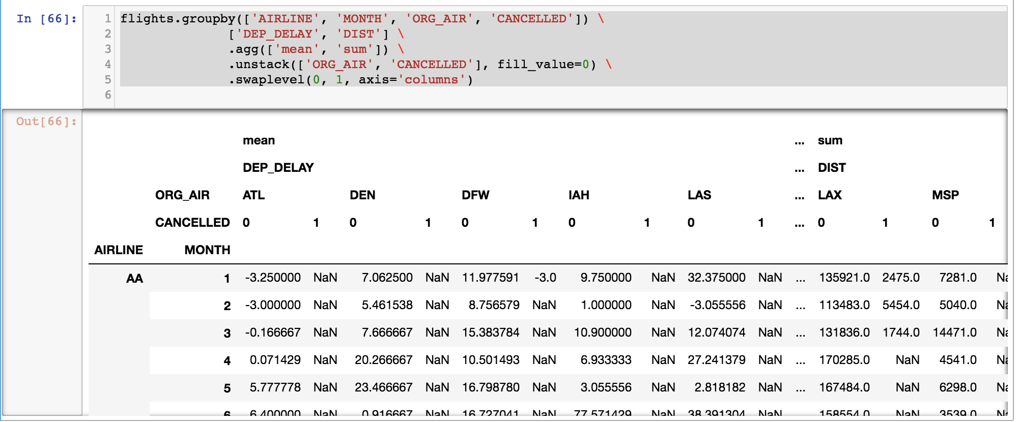
## 给index/columns命名
当我们发现index/columns没有名字时候,可以用
`rename_axis`进行添加,当然需要使用`axis`specify行还是列。
college = pd.read_csv(‘data/college.csv’) cg = college.groupby([‘STABBR’, ‘RELAFFIL’])
[‘UGDS’, ‘SATMTMID’]
.agg([‘size’, ‘min’, ‘max’])
cg.head() # 需要加入columns的名称。 cg = cg.rename_axis([‘AGG_COLS’, ‘AGG_FUNCS’],axis=‘columns’) cg.head() # 把变量AGG_FUNCS放到index中。 cg.stack(‘AGG_FUNCS’).head() # 把’AGG_FUNCS’, ‘STABBR’的位置交换一下。 # swap交换的意思,例如利率交换。 cg.stack(‘AGG_FUNCS’).swaplevel(‘AGG_FUNCS’, ‘STABBR’,axis=‘index’).head() # 这种原数据表的格式看起来乱乱的,因此sort_index一下。 cg.stack(‘AGG_FUNCS’).swaplevel(‘AGG_FUNCS’, ‘STABBR’,axis=‘index’)
.sort_index(level=‘RELAFFIL’, axis=‘index’)
.sort_index(level=‘AGG_COLS’, axis=‘columns’)
.head() # sort_index后,就是一个金字塔结构了,很干净。 # 如果不需要index/columns的名字,可以用None代替。 print cg.rename_axis([None, None], axis=‘index’)
.rename_axis([None, None], axis=‘columns’)
.head()
 UGDS                 SATMTMID
 size    min      max     size    min    max
AK 0 7 109.0 12865.0 7 NaN NaN 1 3 27.0 275.0 3 503.0 503.0 AL 0 72 12.0 29851.0 72 420.0 590.0 1 24 13.0 3033.0 24 400.0 560.0 AR 0 68 18.0 21405.0 68 427.0 565.0
## 文本处理、`split`、`assign`函数和`concat`函数
weightlifting = pd.read_csv(‘data/weightlifting_men.csv’) weightlifting.head() wl_melt = weightlifting.melt(id_vars=‘Weight Category’, var_name = ‘sex_age’, value_name = ‘Qual Total’) # 这样的好处是var_name和value_name至少有我们自定义的名字,不然就叫个value什么的,好屌丝。 # keep going,就是个excel的功能快点。 wl_melt.head() sex_age = wl_melt.sex_age.str.split(expand=True) sex_age.head() sex_age.columns = [‘Sex’, ‘Age Group’] sex_age.head() # 显然我们不要35这个数字,覆盖掉。 sex_age[‘Sex’] = sex_age[‘Sex’].str[0] sex_age.head() wl_cat_total =wl_melt[[‘Weight Category’, ‘Qual Total’]] wl_tidy = pd.concat([sex_age, wl_cat_total], axis=‘columns’) wl_tidy.head() # 这只是第一种方法 # 第二个用正则化表达。 age_group = wl_melt.sex_age.str.extract(’(\d{2}-+?)’, expand=False)
sex = wl_melt.sex_age.str[0] age_group.head() sex.head() new_cols = {‘Sex’:sex, ‘Age Group’: age_group} wl_tidy2 = wl_melt.assign(**new_cols)
.drop(‘sex_age’,axis=‘columns’) print wl_tidy2.sort_index(axis=1).equals(wl_tidy.sort_index(axis=1)) print wl_tidy2.sort_index(axis=1).head()
rue Age Group Qual Total Sex Weight Category 0 35-39 137 M 56 1 35-39 152 M 62 2 35-39 167 M 69 3 35-39 182 M 77 4 35-39 192 M 85
## speead过程columns不要变量名称
inspections = pd.read_csv(‘data/restaurant_inspections.csv’, parse_dates=[‘Date’]) inspections.head() # inspections.pivot( # index = [‘Name’, ‘Date’], # columns = ‘Info’, # values = ‘Value’ # ) # 这是pivot的bug,换另外一种方法 insp_tidy = inspections.set_index([‘Name’,‘Date’,‘Info’])
.unstack(‘Info’)
.reset_index(col_level = -1) insp_tidy # 不要columns的变量名称。 # 这个地方的-1和0,和我们理解idnex顺序一样。 # 现在删除第0行。 insp_tidy.columns = insp_tidy.columns.droplevel(0)
.rename(None) print insp_tidy.head()
Name Date Borough \
0 3 STAR JUICE CENTER 2017-05-10 BROOKLYN
1 A & L PIZZA RESTAURANT 2017-08-22 BROOKLYN
2 AKSARAY TURKISH CAFE AND RESTAURANT 2017-07-25 BROOKLYN
3 ANTOJITOS DELI FOOD 2017-06-01 BROOKLYN
4 BANGIA 2017-06-16 MANHATTAN
Cuisine \
0 Juice, Smoothies, Fruit Salads
1 Pizza
2 Turkish
3 Latin (Cuban, Dominican, Puerto Rican, South &…
4 Korean
Description Grade Score
0 Facility not vermin proof. Harborage or condit… A 12.0
1 Facility not vermin proof. Harborage or condit… A 9.0
2 Plumbing not properly installed or maintained;… A 13.0
3 Live roaches present in facility’s food and/or… A 10.0
4 Covered garbage receptacle not provided or ina… A 9.0
inspections.set_index([‘Name’,‘Date’, ‘Info’])
.squeeze()
.unstack(‘Info’)
.reset_index()
.rename_axis(None, axis=‘columns’) # 这里.squeeze(),就立刻拉平了columns的level,很方便。 # 不需要对0和-1的columns进行修正。
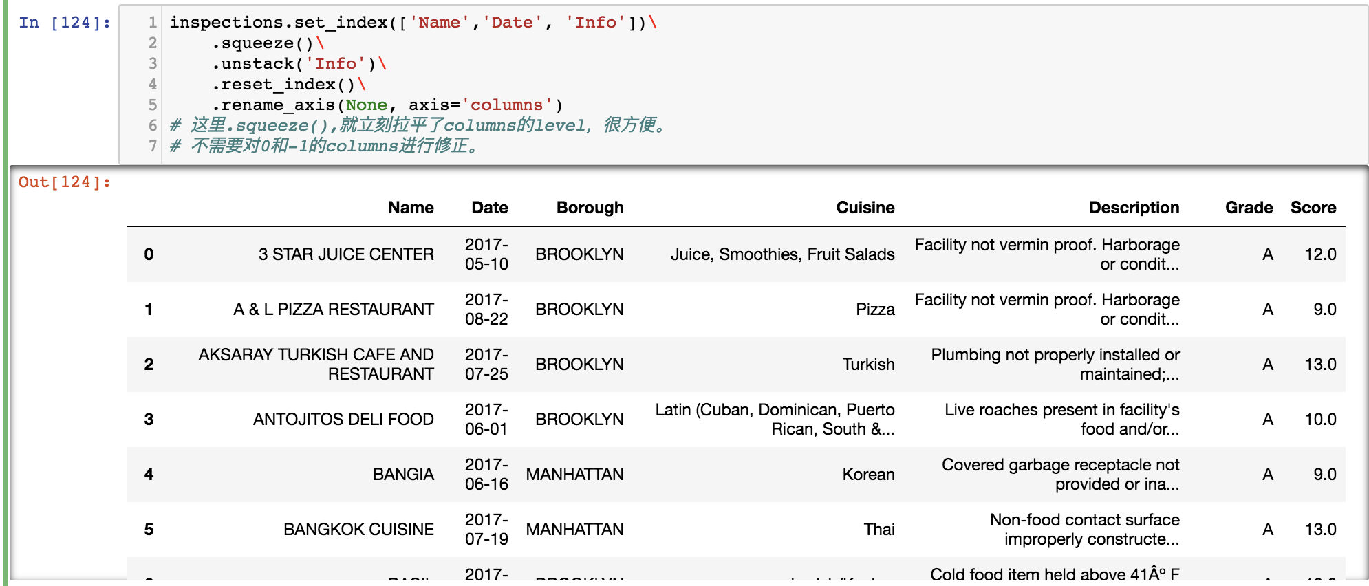
inspections.pivot_table(index=[‘Name’, ‘Date’], columns=‘Info’, values=‘Value’, aggfunc=‘first’)
.reset_index()
.rename_axis(None, axis=‘columns’)
`aggfunc='first'`是考虑重复值的情况,
例如,如果用index和columns发现有重复的,那么选择第一个。

## 文本处理`split`函数
cities = pd.read_csv(‘data/texas_cities.csv’) cities geolocations = cities.Geolocation.str.split(pat=’.’, expand=True) geolocations.columns = [’latitude’, ’latitude direction’, ’longitude’, ’longitude direction’] geolocations = geolocations.apply(pd.to_numeric, errors=‘ignore’) # geolocations = geolocations.astype({’latitude’:‘float’, # ’longitude’:‘float’}) cities_tidy = pd.concat([cities[‘City’], geolocations], axis=‘columns’) print cities_tidy cities.Geolocation.str.split(pat=’° |,’, expand=True) # 这个分的很好, cities.Geolocation.str.extract(’([0-9.]+). (N|S), ([0-9.]+). (E|W)’, expand=True)
City latitude latitude direction longitude longitude direction
0 Houston 29.7604 N 95.3698 W 1 Dallas 32.7767 N 96.7970 W 2 Austin 30.2672 N 97.7431 W
sensors = pd.read_csv(‘data/sensors.csv’) sensors sensors.melt(id_vars=[‘Group’, ‘Property’], var_name=‘Year’)
.head(6) print sensors.melt(id_vars=[‘Group’, ‘Property’], var_name=‘Year’)
.pivot_table(index=[‘Group’, ‘Year’], columns=‘Property’, values=‘value’)
.reset_index()
.rename_axis(None, axis=‘columns’)
.head() # .reset_index()这步,让columns这个变量名称消失,columns的level和index的name变成了一行。 # 最后一行代码是没有意义的,因为reset_index后,就不需要了。 # 第二种方法 print sensors.set_index([‘Group’, ‘Property’])
.stack()
.unstack(‘Property’)
.rename_axis([‘Group’, ‘Year’], axis=‘index’)
.rename_axis(None, axis=‘columns’)
.reset_index()
.head()
Group Year Flow Pressure Temperature 0 A 2012 819 928 1026 1 A 2013 806 873 1038 2 A 2014 861 814 1009 3 A 2015 882 973 1036 4 A 2016 856 870 1042 Group Year Flow Pressure Temperature 0 A 2012 819 928 1026 1 A 2013 806 873 1038 2 A 2014 861 814 1009 3 A 2015 882 973 1036 4 A 2016 856 870 1042
## 分表和合并,table normalizing

这一小节内容多,烦,赶快弄完。
movie = pd.read_csv(‘data/movie_altered.csv’) movie.head() movie.insert(0, ‘id’, np.arange(len(movie))) # insert unique id movie.head() stubnames = [‘director’, ‘director_fb_likes’, ‘actor’, ‘actor_fb_likes’] movie_long = pd.wide_to_long(movie, stubnames=stubnames, i=‘id’, j=‘num’, sep=’_’).reset_index() movie_long[’num’] = movie_long[’num’].astype(int) movie_long.head(9)
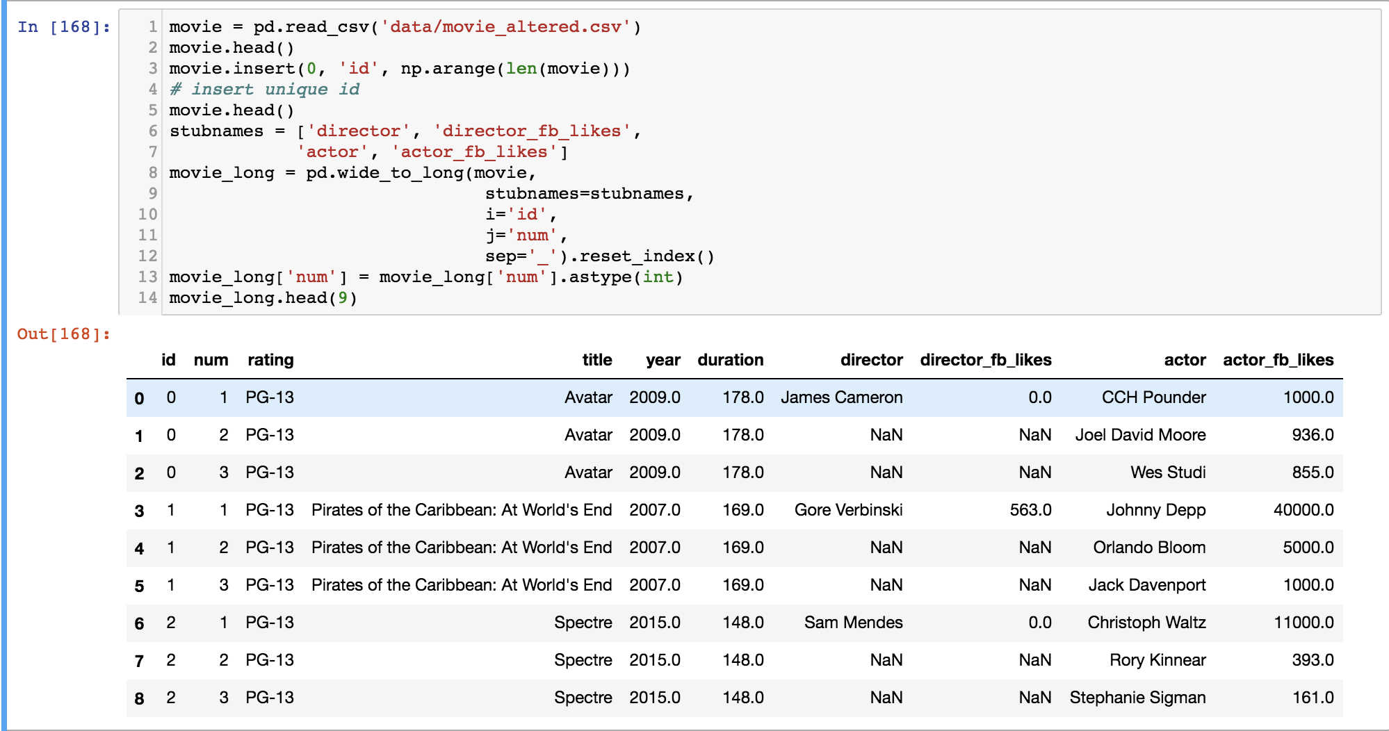
3 table
movie_table = movie_long[[‘id’, ‘year’, ‘duration’, ‘rating’]] director_table = movie_long[[‘id’, ’num’, ‘director’, ‘director_fb_likes’]] actor_table = movie_long[[‘id’, ’num’, ‘actor’, ‘actor_fb_likes’]]
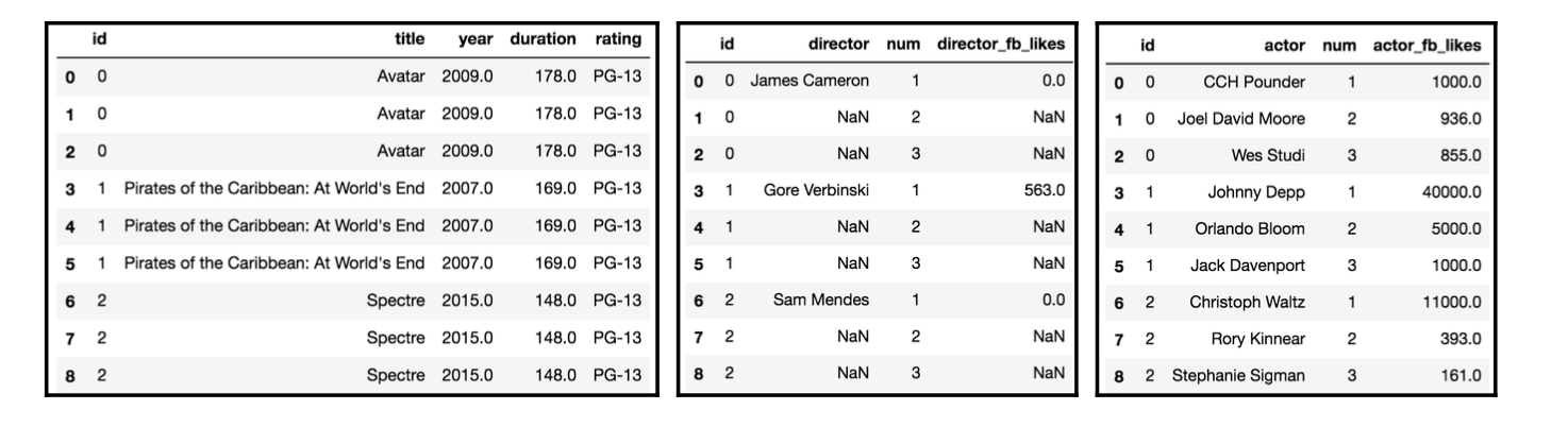
print movie.memory_usage(deep=True).sum() print movie_table.memory_usage(deep=True).sum() +
director_table.memory_usage(deep=True).sum() +
actor_table.memory_usage(deep=True).sum() 1941691 3204490
分表增加了内存。
director_cat = pd.Categorical(director_table[‘director’]) director_table.insert(1, ‘director_id’, director_cat.codes) print director_table.head() actor_cat = pd.Categorical(actor_table[‘actor’]) actor_table.insert(1, ‘actor_id’, actor_cat.codes) print actor_table.head()
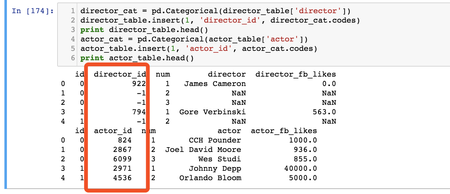
director_associative = director_table[[‘id’, ‘director_id’, ’num’]] dcols = [‘director_id’, ‘director’, ‘director_fb_likes’] director_unique = director_table[dcols].drop_duplicates().reset_index(drop=True) actor_associative = actor_table[[‘id’, ‘actor_id’, ’num’]] acols = [‘actor_id’, ‘actor’, ‘actor_fb_likes’] actor_unique = actor_table[acols].drop_duplicates().reset_index(drop=True) movie_table.memory_usage(deep=True).sum() +
director_associative.memory_usage(deep=True).sum() +
director_unique.memory_usage(deep=True).sum() +
actor_associative.memory_usage(deep=True).sum() +
actor_unique.memory_usage(deep=True).sum() 2165263
现在我们可以把分表重建成大表。
但是是`merge`和`join`的部分了。
现在第八章看完了,这个是拖得最久的,也是最烦的。

# 第九章 SQL

`append`、`concat`、`join`、`merge`。

## `append`的方法
names = pd.read_csv(‘data/names.csv’) names new_data_list = [‘Aria’, 1] names.loc[len(names)] = new_data_list # 这里的len(names),就是dynamic的完成了append。 names # 这里还可以输入文字的,得到non-integer labels. names.loc[‘five’] = new_data_list names names.loc[len(names)] = {‘Name’: ‘Zayd’, ‘Age’: 2} names names.loc[len(names)] = pd.Series({‘Name’: ‘Zayd’, ‘Age’: 2}) names # 所以dict、pd.Series都是可以的。 # 然后开始用append了! names = pd.read_csv(‘data/names.csv’) names.append({‘Name’:‘Aria’, ‘Age’:1}, ignore_index = True) names # 这里的ignore_index类似于覆盖了原来的rangeIndex。 s1 = pd.Series({‘Name’: ‘Zach’, ‘Age’: 3}, name=len(names)) s2 = pd.Series({‘Name’: ‘Zayd’, ‘Age’: 2}, name=‘USA’) # name就是这排pd.Series的index啊,因为append是以行来加入,不是以列,所以不要confuse。 print names.append([s1, s2])
Name Age
0 Cornelia 70 1 Abbas 69 2 Penelope 4 3 Niko 2 4 Zach 3 USA Zayd 2
bball_16 = pd.read_csv(‘data/baseball16.csv’) bball_16.head() # 变量太多,一个个这么打,要跪。 # 因此需要的是,机智的dict方法。 data_dict = bball_16.iloc[0].to_dict() # 找一个例子。 print data_dict # isinstance? # isinstance(A,B)表示是不是A是不是B new_data_dict = {k: ’’ if isinstance(v, str) else np.nan for k, v in data_dict.items()} # 提取key和空values print new_data_dict
{‘2B’: 42, ‘BB’: 60, ‘HR’: 24, ‘IBB’: 11.0, ‘3B’: 5, ‘HBP’: 7.0, ‘GIDP’: 15.0, ‘playerID’: ‘altuvjo01’, ‘stint’: 1, ’teamID’: ‘HOU’, ‘AB’: 640, ‘G’: 161, ‘H’: 216, ‘yearID’: 2016, ‘R’: 108, ‘RBI’: 96.0, ‘CS’: 10.0, ’lgID’: ‘AL’, ‘SH’: 3.0, ‘SO’: 70.0, ‘SB’: 30.0, ‘SF’: 7.0} {‘RBI’: nan, ‘BB’: nan, ‘HR’: nan, ‘IBB’: nan, ‘3B’: nan, ‘stint’: nan, ‘GIDP’: nan, ‘playerID’: ‘’, ‘HBP’: nan, ’teamID’: ‘’, ‘AB’: nan, ‘G’: nan, ‘H’: nan, ‘yearID’: nan, ‘R’: nan, ‘2B’: nan, ‘CS’: nan, ’lgID’: ‘’, ‘SH’: nan, ‘SO’: nan, ‘SB’: nan, ‘SF’: nan}
## `concat`的方法
stocks_2016 = pd.read_csv(‘data/stocks_2016.csv’, index_col=‘Symbol’) stocks_2017 = pd.read_csv(‘data/stocks_2017.csv’, index_col=‘Symbol’) s_list = [stocks_2016, stocks_2017] # 一个list啊,这样理解好!!! pd.concat(s_list) # axis = row是默认的 print pd.concat(s_list, keys = [‘2016test’,‘2017test’]) # 这样没有index的名字 print pd.concat(s_list, keys = [‘2016test’,‘2017test’], names = [‘Year’, ‘Symbol’]) # 后面的’Symbol’本身就有,因此完全是蝙蝠的眼睛。 print pd.concat(s_list,keys = [‘2016’,‘2017’], axis = ‘columns’) # index又没有名字了。 # 这里引入list,那么可以多个inner,不要太好,其实就是一行代码啊!!! # 测试不要太容易。 pd.concat(s_list,keys = [‘2016’,‘2017’], axis = ‘columns’, names = [‘Year’, ‘columns的名字’]) print pd.concat(s_list,keys = [‘2016’,‘2017’], axis = ‘columns’, names = [‘Year’, None]) # 最后inner一下 print pd.concat(s_list,keys = [‘2016’,‘2017’], axis = ‘columns’, names = [‘Year’, None], join = ‘inner’) # 这里只有outer和inner两种
             Shares  Low  High
     Symbol
2016test AAPL 80 95 110 TSLA 50 80 130 WMT 40 55 70 2017test AAPL 50 120 140 GE 100 30 40 IBM 87 75 95 SLB 20 55 85 TXN 500 15 23 TSLA 100 100 300 Shares Low High Year Symbol
2016test AAPL 80 95 110 TSLA 50 80 130 WMT 40 55 70 2017test AAPL 50 120 140 GE 100 30 40 IBM 87 75 95 SLB 20 55 85 TXN 500 15 23 TSLA 100 100 300 2016 2017
Shares Low High Shares Low High AAPL 80.0 95.0 110.0 50.0 120.0 140.0 GE NaN NaN NaN 100.0 30.0 40.0 IBM NaN NaN NaN 87.0 75.0 95.0 SLB NaN NaN NaN 20.0 55.0 85.0 TSLA 50.0 80.0 130.0 100.0 100.0 300.0 TXN NaN NaN NaN 500.0 15.0 23.0 WMT 40.0 55.0 70.0 NaN NaN NaN Year 2016 2017
Shares Low High Shares Low High AAPL 80.0 95.0 110.0 50.0 120.0 140.0 GE NaN NaN NaN 100.0 30.0 40.0 IBM NaN NaN NaN 87.0 75.0 95.0 SLB NaN NaN NaN 20.0 55.0 85.0 TSLA 50.0 80.0 130.0 100.0 100.0 300.0 TXN NaN NaN NaN 500.0 15.0 23.0 WMT 40.0 55.0 70.0 NaN NaN NaN Year 2016 2017
Shares Low High Shares Low High Symbol
AAPL 80 95 110 50 120 140 TSLA 50 80 130 100 100 300
## 爬虫`read_html`略
## `concat`、`merge`和`join`的区别
```
library(DiagrammeR)
grViz(
digraph dot {
graph [layout = dot]
node [shape = egg,
style = filled,
color = darkgreen,
fontsize = 12,
fontname = Helvetica,
fontcolor = white,
# label = ''
]
cb [label = 'combine']
dir [label = 'direction']
dir1 [label = 'horizontally']
dir2 [label = 'vertically']
by [label = 'DataFrame']
by1 [label = 'by index']
by2 [label = 'by columns']
dup [label = 'duplicate']
dup1 [label = 'Errors']
dup2 [label = 'Cartesian prod.']
dft [label = 'default']
dft1 [label = 'outer\nopt. inner']
dft2 [label = 'inner']
dft3 [label = 'left']
edge [
color = darkgreen,
fontsize = 9,
fontname = Helvetica,
fontcolor = dodgerblue,
label = '']
cb -> dir
dir -> dir1 [label = 'concat,join,merge']
dir -> dir2 [label = 'concat']
cb -> by
by -> by1 [label = 'concat']
by -> by2 [label = 'concat,join,merge']
cb -> dup
dup -> dup1 [label = 'concat']
dup -> dup2 [label = 'join,merge']
cb -> dft
dft -> dft1 [label = 'concat']
dft -> dft2 [label = 'merge']
dft -> dft3 [label = 'join']
}")
from IPython.display import display_html
years = 2016, 2017, 2018
stocks_tables = [pd.read_csv('data/stocks_{}.csv'.format(year), index_col = 'Symbol') for year in years]
# 这个可以帮助一次结果,可以展示3个表格在output中,非常实用。
def display_frames(frames, num_spaces=0):
t_style = '<table style="display: inline;"'
tables_html = [df.to_html().replace('<table', t_style)
for df in frames]
space = ' ' * num_spaces
display_html(space.join(tables_html), raw=True)
display_frames(stock_tables, 30)
# 如图就是三个结果。
stocks_2016, stocks_2017, stocks_2018 = stock_tables
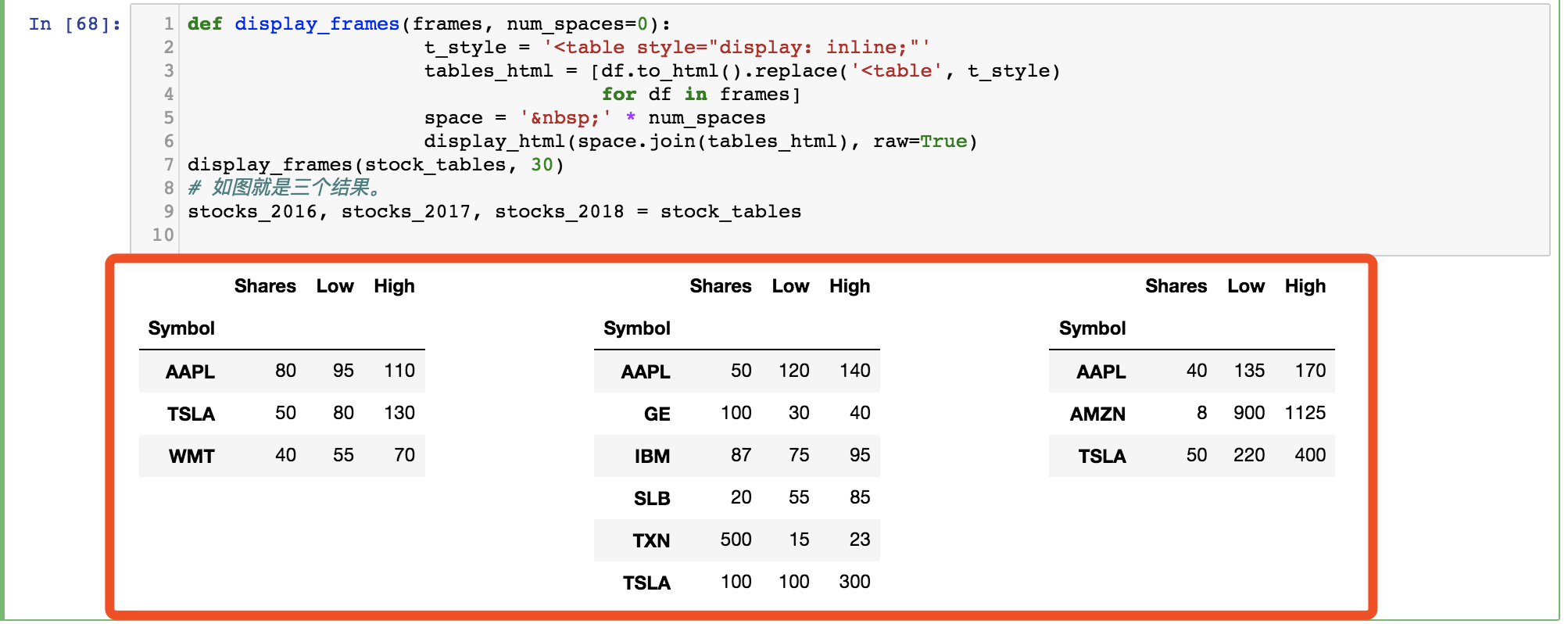
type(stock_tables)
# 因为是list,所以可以直接concat, merge, join.

print pd.concat(stock_tables, keys = [2016,2017,2018])
print pd.concat(stock_tables) # 这样就是没有extra index的。

             Shares  Low  High
     Symbol
2016 AAPL        80   95   110
     TSLA        50   80   130
     WMT         40   55    70
2017 AAPL        50  120   140
     GE         100   30    40
     IBM         87   75    95
     SLB         20   55    85
     TXN        500   15    23
     TSLA       100  100   300
2018 AAPL        40  135   170
     AMZN         8  900  1125
     TSLA        50  220   400
        Shares  Low  High
Symbol
AAPL        80   95   110
TSLA        50   80   130
WMT         40   55    70
AAPL        50  120   140
GE         100   30    40
IBM         87   75    95
SLB         20   55    85
TXN        500   15    23
TSLA       100  100   300
AAPL        40  135   170
AMZN         8  900  1125
TSLA        50  220   400

print zip(years,stock_tables)
print dict(zip(years,stock_tables))
# 一个是zip list
# 一个是dict

[(2016,         Shares  Low  High
Symbol
AAPL        80   95   110
TSLA        50   80   130
WMT         40   55    70), (2017,         Shares  Low  High
Symbol
AAPL        50  120   140
GE         100   30    40
IBM         87   75    95
SLB         20   55    85
TXN        500   15    23
TSLA       100  100   300), (2018,         Shares  Low  High
Symbol
AAPL        40  135   170
AMZN         8  900  1125
TSLA        50  220   400)]

{2016:         Shares  Low  High
Symbol
AAPL        80   95   110
TSLA        50   80   130
WMT         40   55    70, 2017:         Shares  Low  High
Symbol
AAPL        50  120   140
GE         100   30    40
IBM         87   75    95
SLB         20   55    85
TXN        500   15    23
TSLA       100  100   300, 2018:         Shares  Low  High
Symbol
AAPL        40  135   170
AMZN         8  900  1125
TSLA        50  220   400}

print pd.concat(dict(zip(years,stock_tables)), axis='columns')
# axis='columns' 这个方向我就不想说了,简单。
# 因此横向合并实际上,需要list化加上dict化的
# 这样可以产生columns里面第一级的index
不然的话,需要加变量后缀,类似于type.x或type.y
       2016                2017                 2018
     Shares   Low   High Shares    Low   High Shares    Low    High
AAPL   80.0  95.0  110.0   50.0  120.0  140.0   40.0  135.0   170.0
AMZN    NaN   NaN    NaN    NaN    NaN    NaN    8.0  900.0  1125.0
GE      NaN   NaN    NaN  100.0   30.0   40.0    NaN    NaN     NaN
IBM     NaN   NaN    NaN   87.0   75.0   95.0    NaN    NaN     NaN
SLB     NaN   NaN    NaN   20.0   55.0   85.0    NaN    NaN     NaN
TSLA   50.0  80.0  130.0  100.0  100.0  300.0   50.0  220.0   400.0
TXN     NaN   NaN    NaN  500.0   15.0   23.0    NaN    NaN     NaN
WMT    40.0  55.0   70.0    NaN    NaN    NaN    NaN    NaN     NaN

print stocks_2016.join(stocks_2017,lsuffix='_2016',rsuffix='_2017', how = 'outer')

        Shares_2016  Low_2016  High_2016  Shares_2017  Low_2017  High_2017
Symbol
AAPL           80.0      95.0      110.0         50.0     120.0      140.0
GE              NaN       NaN        NaN        100.0      30.0       40.0
IBM             NaN       NaN        NaN         87.0      75.0       95.0
SLB             NaN       NaN        NaN         20.0      55.0       85.0
TSLA           50.0      80.0      130.0        100.0     100.0      300.0
TXN             NaN       NaN        NaN        500.0      15.0       23.0
WMT            40.0      55.0       70.0          NaN       NaN        NaN

print stocks_2017.add_suffix('_2017')
# 在确定好用的时候,只会用到index来合并,所有columns都是需要的变量,那么直接加后缀就好。

        Shares_2017  Low_2017  High_2017
Symbol
AAPL             50       120        140
GE              100        30         40
IBM              87        75         95
SLB              20        55         85
TXN             500        15         23
TSLA            100       100        300

other = [stocks_2017.add_suffix('_2017'),
            stocks_2018.add_suffix('_2018')]
print stocks_2016.add_suffix('_2016').join(other, how='outer')

      Shares_2016  Low_2016  High_2016  Shares_2017  Low_2017  High_2017  \
AAPL         80.0      95.0      110.0         50.0     120.0      140.0
AMZN          NaN       NaN        NaN          NaN       NaN        NaN
GE            NaN       NaN        NaN        100.0      30.0       40.0
IBM           NaN       NaN        NaN         87.0      75.0       95.0
SLB           NaN       NaN        NaN         20.0      55.0       85.0
TSLA         50.0      80.0      130.0        100.0     100.0      300.0
TXN           NaN       NaN        NaN        500.0      15.0       23.0
WMT          40.0      55.0       70.0          NaN       NaN        NaN

      Shares_2018  Low_2018  High_2018
AAPL         40.0     135.0      170.0
AMZN          8.0     900.0     1125.0
GE            NaN       NaN        NaN
IBM           NaN       NaN        NaN
SLB           NaN       NaN        NaN
TSLA         50.0     220.0      400.0
TXN           NaN       NaN        NaN
WMT           NaN       NaN        NaN

stock_join = stocks_2016.add_suffix('_2016').join(other,
                                                           how='outer')
stock_concat = pd.concat(dict(zip(years,stock_tables)),
                                  axis='columns')
level_1 = stock_concat.columns.get_level_values(1)

level_0 = stock_concat.columns.get_level_values(0).astype(str)
stock_concat.columns = level_1 + '_' + level_0
stock_join.equals(stock_concat)
True

step1 = stocks_2016.merge(stocks_2017, left_index=True,
                                   right_index=True, how='outer',
                                   suffixes=('_2016', '_2017'))
stock_merge = step1.merge(stocks_2018.add_suffix('_2018'),
                                   left_index=True, right_index=True,
                                   how='outer')
stock_concat.equals(stock_merge)
True

# 我们发现前面都是靠index进行合并的,用到了*_index。
# 现在对变量进行on
names = ['prices', 'transactions']
food_tables = [pd.read_csv('data/food_{}.csv'.format(name))
                         for name in names]
food_prices, food_transactions = food_tables
display_frames(food_tables, 30)
print food_tables

[     item store  price  Date
0    pear     A   0.99  2017
1    pear     B   1.99  2017
2   peach     A   2.99  2017
3   peach     B   3.49  2017
4  banana     A   0.39  2017
5  banana     B   0.49  2017
6   steak     A   5.99  2017
7   steak     B   6.99  2017
8   steak     B   4.99  2015,    custid     item store  quantity
0       1     pear     A         5
1       1   banana     A        10
2       2    steak     B         3
3       2     pear     B         1
4       2    peach     B         2
5       2    steak     B         1
6       2  coconut     B         4]

print food_transactions.merge(food_prices, on = ["item","store"])
   custid    item store  quantity  price  Date
0       1    pear     A         5   0.99  2017
1       1  banana     A        10   0.39  2017
2       2   steak     B         3   6.99  2017
3       2   steak     B         3   4.99  2015
4       2   steak     B         1   6.99  2017
5       2   steak     B         1   4.99  2015
6       2    pear     B         1   1.99  2017
7       2   peach     B         2   3.49  2017
默认是inner
# 尝试left,加上how
print food_transactions.merge(food_prices.query('Date == 2017'),
                                  how='left')

   custid     item store  quantity  price    Date
0       1     pear     A         5   0.99  2017.0
1       1   banana     A        10   0.39  2017.0
2       2    steak     B         3   6.99  2017.0
3       2     pear     B         1   1.99  2017.0
4       2    peach     B         2   3.49  2017.0
5       2    steak     B         1   6.99  2017.0
6       2  coconut     B         4    NaN     NaN

pd.concat([food_transactions.set_index(['item', 'store']),
                           food_prices.set_index(['item', 'store'])],
                          axis='columns')
Exception: cannot handle a non-unique multi-index!
blob批量操作,省略for循环
import glob
df_list = []
for filename in glob.glob('data/gas prices/*.csv'):
    df_list.append(pd.read_csv(filename, index_col='Week',
                          parse_dates=['Week']))
gas = pd.concat(df_list, axis='columns')
gas.head()

            All Grades  Diesel  Midgrade  Premium  Regular
Week
2017-09-25       2.701   2.788     2.859    3.105    2.583
2017-09-18       2.750   2.791     2.906    3.151    2.634
2017-09-11       2.800   2.802     2.953    3.197    2.685
2017-09-04       2.794   2.758     2.946    3.191    2.679
2017-08-28       2.513   2.605     2.668    2.901    2.399
链接数据库
from sqlalchemy import create_engine
engine = create_engine('sqlite:///data/chinook.db')
tracks = pd.read_sql_table('tracks',engine)
print tracks.head()
genres = pd.read_sql_table('genres',engine)
print genres.head()
# display_frames([genres,tracks], 30)

   TrackId                                     Name  AlbumId  MediaTypeId  \
0        1  For Those About To Rock (We Salute You)        1            1
1        2                        Balls to the Wall        2            2
2        3                          Fast As a Shark        3            2
3        4                        Restless and Wild        3            2
4        5                     Princess of the Dawn        3            2

   GenreId                                           Composer  Milliseconds  \
0        1          Angus Young, Malcolm Young, Brian Johnson        343719
1        1                                               None        342562
2        1  F. Baltes, S. Kaufman, U. Dirkscneider & W. Ho...        230619
3        1  F. Baltes, R.A. Smith-Diesel, S. Kaufman, U. D...        252051
4        1                         Deaffy & R.A. Smith-Diesel        375418

      Bytes  UnitPrice
0  11170334       0.99
1   5510424       0.99
2   3990994       0.99
3   4331779       0.99
4   6290521       0.99
   GenreId                Name
0        1                Rock
1        2                Jazz
2        3               Metal
3        4  Alternative & Punk
4        5       Rock And Roll

print genres.merge(tracks[['GenreId','Milliseconds']], on = 'GenreId', how = 'left')\
    .drop('GenreId',axis = 'columns')\
    .head()
# 把key删除了

   Name  Milliseconds
0  Rock        343719
1  Rock        342562
2  Rock        230619
3  Rock        252051
4  Rock        375418

genre_track = genres.merge(tracks[['GenreId','Milliseconds']], on = 'GenreId', how = 'left')\
    .drop('GenreId',axis = 'columns')
print genre_track.head()
# 把key删除了
genre_time = genre_track.groupby('Name')['Milliseconds'].mean()
genre_time.head()
pd.to_timedelta(genre_time, unit='ms').dt.floor('s').sort_values().head()
# 这里转换时间我不太懂,之后看时间序列的时候再注意。

Name
Rock And Roll    00:02:14
Opera            00:02:54
Hip Hop/Rap      00:02:58
Easy Listening   00:03:09
Bossa Nova       00:03:39
Name: Milliseconds, dtype: timedelta64[ns]

# 多个表连续合并
cust = pd.read_sql_table('customer', engine, columns = ['CustomerId','FirstName','LastName'])
invoice = pd.read_sql_table('invoices', engine, columns=['InvoiceId','CustomerId'])
ii = pd.read_sql_table('invoice_items', engine, columns=['InvoiceId', 'UnitPrice','Quantity'])
cust_inv = cust.merge(invoice, on='CustomerId') \
                        .merge(ii, on='InvoiceId')
cust_inv.head()
总结
create_engine需要一个connection string,涵盖了数据库的位置。 复杂的需要, dialect+driver://username:password@host:port/database 。
可以尝试下pd.read_sql_query。
pd.read_sql_query(sql_string1, engine) 这样就可以了。