Unsupervised Learning in Python 学习笔记

Unsupervised Learning in Python

网页在这。 是这个哥们教的， Benjamin Wilson | DataCamp 。 主要讲了一部分基本的特征工程的东西，比R课讲得清楚， 很可惜这个老师datacamp只有这门课， 相对来说，教Python的，理论部分是要清楚很多。 涉及PCA、KMeans、NMF，还不错。

提到 dimension reduction 降维。 主成分？ 聚类？

没有prediction task，就是为了clustering。

用到k-means clustering with scikit-learn。

k-means还可以做预测，因为它记得住之前计算好的means，即centroids ¹。

slides下载不了，只能抗推了。

Clustering 2D points | Python

# Import KMeans
from sklearn.cluster import KMeans

# Create a KMeans instance with 3 clusters: model
model = KMeans(n_clusters = 3)

# Fit model to points
model.fit(points)

# Determine the cluster labels of new_points: labels
labels = model.predict(new_points)

# Print cluster labels of new_points
print(labels)

model = KMeans(n_clusters = 3)先把模型看成一个对象。 使用对象去fit模型，直接那么写 model.fit(points)，真尴尬。 最后预测模型，用model.predict(new_points) 因此如果要算老样本的\hat y，其实也是要用model.predict()的。 但是这个地方是model.predict(points)。

Inspect your clustering | Python

# Import pyplot
import matplotlib.pyplot as plt

# Assign the columns of new_points: xs and ys
xs = new_points[:,0]
ys = new_points[:,1]

# Make a scatter plot of xs and ys, using labels to define the colors
plt.scatter(xs, ys, c = labels, alpha = 0.5)

# Assign the cluster centers: centroids
centroids = model.cluster_centers_

# Assign the columns of centroids: centroids_x, centroids_y
centroids_x = centroids[:,0]
centroids_y = centroids[:,1]

# Make a scatter plot of centroids_x and centroids_y
plt.scatter(centroids_x, centroids_y, marker = 'D', s = 50)
plt.show()

这个地方看图就知道，质心的理解了。 另外，model.cluster_centers_这个代码是告诉质心的坐标。 现在知道model.predict怎么估计的了，质心知道了，根据input的特性，离哪个质心近，哪个就对就好了。

但是具体选多少个质心，这个之后讨论。

这里很衡量了如何使用forloop进行KMeans最佳质心选取，选取标准是elbow最优。

K均值聚类（理论部分）

K均值是基于距离计算的，从中心点搜寻周围近的其他点，所以是类球形的点适合这样的算法。最好是要对原始数据作异常值检验。

这个总结的很好。

以欧氏距离为例，

\[D = ((x_1-x_2)^2 + (y_1 - y_2)^2 )^{\frac{1}{2}}\]

步骤：

• 在n个观测中随机挑选K个观测，每个观测代表一个簇；
• 计算剩余的每个对象到各个簇的欧式距离，将他们分配到最相近的簇中，并计算新簇的均值；
• 使用新的均值作为新簇的中心，再重新分配所有对象，计算簇均值
• 重复第二步和第三步,直到分配稳定，形成最终的k个类。

使用新的均值作为新簇的中心，就是这个地方理解的关键了，其他都无所谓。

损失函数定义

\[SSE = \sum_{j=1}^{K} \sum_{i=1}^{N_{j}}((x_i-\mu_j)^2)\]

\(SSE\)使得最小。 其中\(\mu_j\)表示第\(j\)个簇的均值向量，这里的\(x\)也是向量！！！ 因此这里有\(K\)个簇。 在第\(j\)个簇里面，包含了\(N_{j}\)个样本。

就是这个意思。

然后下面一阶偏导出最优化条件。

矩阵求导看这个，* 正则化理解 - A Hugo website。

$$

\[\begin{alignat}{2} \frac{\partial SSE}{\partial \mu_{j}} & = \frac{\partial}{\partial \mu_j} \sum_{j=1}^{K} \sum_{i=1}^{N_{j}}((x_i-\mu_j)^2) \\ & = \sum_{j=1}^{K} \sum_{i=1}^{N_{j}} \frac{\partial}{\partial \mu_j} ((x_i-\mu_j)^2) \\ & = \sum_{i=1}^{N_{j}} -\frac{\partial}{\partial \mu_j} ((x_i-\mu_j)) \\ & = 0 \\ & \to \mu_j = \frac{1}{N_j} \sum_{i=1}^{N_j}x_j \end{alignat}\] $$

这个最优化的结果就是计算簇的均值！

Evaluating a clustering | Python

这个地方，因为我们已知了只有三种物种，所以我们当然知道n_clusters = 3。 但是引发了一个新问题，我们既然也是分三类，是否可以用混合矩阵来看看准确率？ 这个是pd.crosstab()的作用。

Inertia ² 衡量了KMeans的效果，就是每个小分类中，样本离质心的距离和。

在model.fit(samples)后，model.inertia来发现。

看到图，就知道了，clusters越多，inertia越小，但是衰减速度下降了。

elbow ³ 就是衡量下降速率下降的问题。

接下来，可以通过for loop解决这个问题。

How many clusters of grain? | Python

ks = range(1, 6)
inertias = []

for k in ks:
    # Create a KMeans instance with k clusters: model
    model = KMeans(n_clusters = k)
    
    # Fit model to samples
    model.fit(samples)
    
    # Append the inertia to the list of inertias
    inertias.append(model.inertia_)
    
# Plot ks vs inertias
plt.plot(ks, inertias, '-o')
plt.xlabel('number of clusters, k')
plt.ylabel('inertia')
plt.xticks(ks)
plt.show()

Evaluating the grain clustering | Python

# Create a KMeans model with 3 clusters: model
model = KMeans(n_clusters = 3)

# Use fit_predict to fit model and obtain cluster labels: labels
labels = model.fit_predict(samples)

# Create a DataFrame with labels and varieties as columns: df
df = pd.DataFrame({'labels': labels, 'varieties': varieties})

# Create crosstab: ct
ct = pd.crosstab(df['labels'],df['varieties'])

# Display ct
print(ct)

fit_predict这里合并和.fit和.predict(oldsample)。

<script.py> output:
    varieties  Canadian wheat  Kama wheat  Rosa wheat
    labels                                           
    0                      68           9           0
    1                       0           1          60
    2                       2          60          10

Transforming features for better clusterings | Python

StandardScalar就是标准化，所谓的标准化就是\(\mu = 0\)和\(\sigma = 1\)。

\[\tilde x = \frac{x-\bar x}{\sigma_x}\]

\[E(\tilde x) = E(\frac{x-\bar x}{\sigma_x}) = E(\frac{x}{\sigma_x})-E(\frac{\bar x}{\sigma_x})=0\]

\[Var(\tilde x) = Var(\frac{x-\bar x}{\sigma_x}) = \frac{1}{\sigma_{x}^2} \cdot Var(x-\bar x) = \frac{Var(x)}{\sigma_{x}^2} = 1\]

from sklearn.preprocessing import StandardScalar引入。

并且，当然是先标准化后KMeans，因此这里可以引入pipeline。 from sklearn.pipeline import make_pipeline 。

的确标准化可以改善KMeans的分类能力。

\(\Box\)还要其他的方法 MaxAbsScaler和Normalizer，这个可以回家看看。

Scaling fish data for clustering | Python

sklearn包其实有书，这里可以看， 有没有讲sklearn的书？ - 知乎 。

Hands-On Machine Learning with Scikit-Learn and TensorFlow: Concepts, Tools, and Techniques to Build Intelligent Systems: Aurélien Géron: 9781491962299: Amazon.com: Books 这个应该好，但是没时间看，先放着。

当我们需要将特征值都归一化为某个范围[a,b]时，选MinMaxScaler ⁴, 当我们需要归一化后的特征值均值为0，标准差为1，选StandardScaler

标准化与归一化的区别

简单来说，标准化是依照特征矩阵的列处理数据，其通过求z-score的方法，将样本的特征值转换到同一量纲下。归一化是依照特征矩阵的行处理数据，其目的在于样本向量在点乘运算或其他核函数计算相似性时，拥有统一的标准，也就是说都转化为“单位向量” ⁵。规则为l2的归一化公式如下：

\[\tilde x = \frac{x}{|x|}\]

\[|x| = \sum_{i=1}^mx_i\]

其中\(x\)表示一个行向量，即一个用户的数据。 \(m\)表示有m个特征。

机器学习中，有哪些特征选择的工程方法？ - 知乎

在Python中的一个例子。

import numpy as np
raw = [0.07, 0.14, 0.07]
sum = []
for i in raw:
    i2 = i ** 2
    sum.append(i2)
sum_2 = np.sum(sum) ** 0.5
norm = raw / sum_2
print(norm)

# Perform the necessary imports
from sklearn.pipeline import make_pipeline
from sklearn.preprocessing import StandardScaler
from sklearn.cluster import KMeans

# Create scaler: scaler
scaler = StandardScaler()

# Create KMeans instance: kmeans
kmeans = KMeans(n_clusters = 4)

# Create pipeline: pipeline
pipeline = make_pipeline(scaler, kmeans)

先把pipe写好。

Clustering the fish data | Python

samples is the 2D array of fish measurements.

注意啊逗比，这个地方说的是二维矩阵，不是只有两个变量。

In [2]: samples[:5,]
Out[2]: 
array([[ 242. ,   23.2,   25.4,   30. ,   38.4,   13.4],
       [ 290. ,   24. ,   26.3,   31.2,   40. ,   13.8],
       [ 340. ,   23.9,   26.5,   31.1,   39.8,   15.1],
       [ 363. ,   26.3,   29. ,   33.5,   38. ,   13.3],
       [ 430. ,   26.5,   29. ,   34. ,   36.6,   15.1]])

就是一个table。

# Import pandas
import pandas as pd

# Fit the pipeline to samples
pipeline.fit(samples)

# Calculate the cluster labels: labels
labels = pipeline.predict(samples)

# Create a DataFrame with labels and species as columns: df
df = pd.DataFrame({'labels': labels, 'species': species})

# Create crosstab: ct
ct = pd.crosstab(df['labels'], df['species'])

# Display ct
print(ct)

labels是预测值， species是真实值， 因此比较比较。

species  Bream  Pike  Roach  Smelt
labels                            
0            1     0     19      1
1            0    17      0      0
2           33     0      1      0
3            0     0      0     13

还可以。

Clustering stocks using KMeans | Python

Normalizer() rescales each sample - here, each company’s stock price - independently of the other.

因为都是单位向量，都有自己独立的方向。

# Import Normalizer
from sklearn.preprocessing import Normalizer

# Create a normalizer: normalizer
normalizer = Normalizer()

# Create a KMeans model with 10 clusters: kmeans
kmeans = KMeans(n_clusters = 10)

# Make a pipeline chaining normalizer and kmeans: pipeline
pipeline = make_pipeline(normalizer, kmeans)

# Fit pipeline to the daily price movements
pipeline.fit(movements)

Which stocks move together? | Python

# Import pandas
import pandas as pd

# Predict the cluster labels: labels
labels = pipeline.predict(movements)

# Create a DataFrame aligning labels and companies: df
df = pd.DataFrame({'labels': labels, 'companies': companies})

# Display df sorted by cluster label
print(df.sort_values('labels'))

对啊，这个就可以看走势了！ 哪些是一个方向的。

                             companies  labels
20                          Home Depot       0
0                                Apple       1
22                                  HP       1
13                   DuPont de Nemours       1
12                             Chevron       1
23                                 IBM       1
10                      ConocoPhillips       1
8                          Caterpillar       1
35                            Navistar       1
43                                 SAP       1
44                        Schlumberger       1
53                       Valero Energy       1
57                               Exxon       1
32                                  3M       1
16                   General Electrics       1
30                          MasterCard       2
36                    Northrop Grumman       2
29                     Lookheed Martin       2
4                               Boeing       2
40                      Procter Gamble       3
56                            Wal-Mart       3
25                   Johnson & Johnson       3
27                      Kimberly-Clark       3
54                            Walgreen       3
39                              Pfizer       3
9                    Colgate-Palmolive       3
17                     Google/Alphabet       4
47                            Symantec       4
50  Taiwan Semiconductor Manufacturing       4
33                           Microsoft       4
51                   Texas instruments       4
59                               Yahoo       4
24                               Intel       4
11                               Cisco       4
14                                Dell       4
2                               Amazon       4
58                               Xerox       4
15                                Ford       5
1                                  AIG       5
55                         Wells Fargo       6
3                     American express       6
18                       Goldman Sachs       6
5                      Bank of America       6
26                      JPMorgan Chase       6
34                          Mitsubishi       7
45                                Sony       7
21                               Honda       7
48                              Toyota       7
7                                Canon       7
19                     GlaxoSmithKline       8
52                            Unilever       8
42                   Royal Dutch Shell       8
49                               Total       8
6             British American Tobacco       8
46                      Sanofi-Aventis       8
37                            Novartis       8
31                           McDonalds       9
28                           Coca Cola       9
41                       Philip Morris       9
38                               Pepsi       9

马德真多，画图画图！

Visualizing hierarchies | Python

视频下载，推荐迅雷下载，直接粘贴链接进去，我试过百度云，貌似不行。

https://videos.datacamp.com/transcoded_mp4/2072_unsupervised_learning/v1/ch2_1.mp4
https://videos.datacamp.com/transcoded_mp4/2072_unsupervised_learning/v1/ch2_2.mp4
https://videos.datacamp.com/transcoded_mp4/2072_unsupervised_learning/v1/ch2_3.mp4

Hierarchical clustering:

• Every country begins in a separate cluster
• At each step, the two closest clusters are merged
• Continue until all countries in a single cluster
• This is “agglomerative” ⁶ hierarchical clustering

from scipy.cluster.hierarchy import linkage, dendrogram引入 ^{7 8}。

Hierarchical clustering of the grain data | Python

书签，好困，早上起来做，哈哈。

linkage(samples, method = 'complete')中 method = 'complete'表示

In [7]: help(linkage)
Help on function linkage in module scipy.cluster.hierarchy:

linkage(y, method='single', metric='euclidean')
      * method='complete' assigns
    
        .. math::
           d(u, v) = \max(dist(u[i],v[j]))
    
        for all points :math:`i` in cluster u and :math:`j` in
        cluster :math:`v`. This is also known by the Farthest Point
        Algorithm or Voor Hees Algorithm.

In [8]: type(samples)
Out[8]: numpy.ndarray

In [14]: samples.shape
Out[14]: (42, 7)

# Perform the necessary imports
from scipy.cluster.hierarchy import linkage, dendrogram
import matplotlib.pyplot as plt

# Calculate the linkage: mergings
mergings = linkage(samples, method = 'complete')

# Plot the dendrogram, using varieties as labels
dendrogram(mergings,
           labels=varieties,
           leaf_rotation=90,
           leaf_font_size=6,
)
plt.show()

labels=varieties其中varieties是给定好的np.array，ID名称。

varieties的情况如下：

In [10]: set(varieties)
Out[10]: {'Canadian wheat', 'Kama wheat', 'Rosa wheat'}

leaf_rotation就是文字转向。

Hierarchies of stocks | Python

# Import normalize
from sklearn.preprocessing import normalize

# Normalize the movements: normalized_movements
normalized_movements = normalize(movements)

# Calculate the linkage: mergings
mergings = linkage(normalized_movements, method = 'complete')

# Plot the dendrogram
dendrogram(mergings, labels = companies, leaf_rotation=90, leaf_font_size=6)
plt.show()

本身这个办法可以用来理解，n_clusters具体怎么分配的。

Cluster labels in hierarchical clustering | Python

终于理解那个图的高度了，其实就是样本间的距离。

Height on dendrogram = distance between merging clusters

Height on dendrogram specifies max. distance between merging clusters

这就是为什么linkage中method = 'complete'的定义是max(a,b)。

Defined by a “linkage method”

Specified via method parameter, e.g. linkage(samples, method="complete")

In “complete” linkage: distance between clusters is max. distance between their samples

Different linkage method, different hierarchical clustering!

指定特定的距离，标记label。

from scipy.cluster.hierarchy import linkage导入。

mergings = linkage(samples, method='complete')计算距离。

from scipy.cluster.hierarchy import fcluster导入。

labels = fcluster(mergings, 15, criterion='distance')中15是特定的距离。

然后将labels和country_names合并，召唤pandas，import pandas as pd。

pairs = pd.DataFrame({'labels': labels, 'countries': country_names})
print(pairs.sort_values('labels'))

Different linkage, different hierarchical clustering! | Python

method='single'使用，而不是method='complete'。

# Perform the necessary imports
import matplotlib.pyplot as plt
from scipy.cluster.hierarchy import linkage, dendrogram

# Calculate the linkage: mergings
mergings = linkage(samples, method = 'single')

# Plot the dendrogram
dendrogram(mergings, labels = country_names, leaf_rotation=90, leaf_font_size=6)
plt.show()

Extracting the cluster labels | Python

# Perform the necessary imports
import pandas as pd
from scipy.cluster.hierarchy import fcluster

# Use fcluster to extract labels: labels
labels = fcluster(mergings, 6, criterion='distance')

# Create a DataFrame with labels and varieties as columns: df
df = pd.DataFrame({'labels': labels, 'varieties': varieties})

# Create crosstab: ct
ct = pd.crosstab(df['labels'], df['varieties'])

# Display ct
print(ct)

<script.py> output:
    varieties  Canadian wheat  Kama wheat  Rosa wheat
    labels                                           
    1                      14           3           0
    2                       0           0          14
    3                       0          11           0

t-SNE for 2-dimensional maps | Python

t-SNE = “t-distributed stochastic neighbor embedding” 这是t-SNE的全称，主要用于高维数据可视化。高维数据，表示一个用户数据，可以用10个、100个维度去描述，也就是特征多，这个时候，为了跟业务部门展示数据的分类， t-SNE就发挥了这样的作用。

这个图可以感受一下，

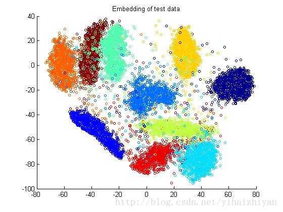
Python中， from sklearn.manifold import TSNE引入。 .fit_transform, simultaneously fits the model and transforms the data, Can’t extend the map to include new data samples. learning_rate=100, try values between 50 and 200

徐志强: t-sne是流行学习的一种，属于非线性降维的一种，主要是保证高维空间中相似的数据点在低维空间中尽量挨得近。是从sne演化而来，sne中用高斯分布衡量高维和地位空间数据点之间的相似性，t-sne主要是为了解决sne中的“拥挤问题”，用t分布定义低维空间低维空间中点的相似性。但是t-sne不能算是一种通用的降维方法吧，时间复杂度也挺高的。

t-SNE visualization of grain dataset | Python

from sklearn.manifold import TSNE引入。⁹

# Import TSNE
from sklearn.manifold import TSNE

# Create a TSNE instance: model
model = TSNE(learning_rate = 200)

# Apply fit_transform to samples: tsne_features
tsne_features = model.fit_transform(samples)

# Select the 0th feature: xs
xs = tsne_features[:,0]

# Select the 1st feature: ys
ys = tsne_features[:,1]

# Scatter plot, coloring by variety_numbers
plt.scatter(xs, ys, c = variety_numbers)
plt.show()

其中tsne_features是产生的一个\(N \times 2\)向量。

In [4]: tsne_features.shape
Out[4]: (210, 2)

A t-SNE map of the stock market | Python

# Import TSNE
from sklearn.manifold import TSNE 

# Create a TSNE instance: model
model = TSNE(learning_rate = 50)

# Apply fit_transform to normalized_movements: tsne_features
tsne_features = model.fit_transform(normalized_movements)

# Select the 0th feature: xs
xs = tsne_features[:,0]

# Select the 1th feature: ys
ys = tsne_features[:,1]

# Scatter plot
plt.scatter(xs, ys, alpha=0.5)

# Annotate the points
for x, y, company in zip(xs, ys, companies):
    plt.annotate(company, (x, y), fontsize=5, alpha=0.75)
plt.show()

相似的变量靠的近。

Visualizing the PCA transformation | Python

开始讲主成分分析， 开始讲降维了。

Dimension reduction

PCA = “Principal Component Analysis” , Fundamental dimension reduction technique ,

• First step “decorrelation” (considered here) ,
• Second step reduces dimension (considered later)

转置样本，平行于坐标轴，使得样本的均值为0， 没有信息损失。

因此， PCA a scikit-learn component like KMeans or StandardScaler.

fit() learns the transformation from given data

• transform() applies the learned transformation
• transform() can also be applied to new data

主成分分析的主要特点 原样本的特征是相关的，但是在PCA中，因为数据是依靠着坐标轴， 因此PCA的特征是不线性相关的，因此是n. 解[抗,去]相关。 可以用Pearson系数检验。

“Principal components” = directions of variance, PCA aligns principal components with the axes, Available as components_ attribute of PCA object.

所以每一行的均值为0。

Correlated data in nature | Python

# Perform the necessary imports
import matplotlib.pyplot as plt
from scipy.stats import pearsonr

# Assign the 0th column of grains: width
width = grains[:,0]

# Assign the 1st column of grains: length
length = grains[:,1]

# Scatter plot width vs length
plt.scatter(width, length)
plt.axis('equal')
plt.show()

# Calculate the Pearson correlation
correlation, pvalue = pearsonr(width, length)

# Display the correlation
print(correlation)

Decorrelating the grain measurements with PCA | Python

看到图就知道了，的确\(\rho=0\)且\(\mu = 0\)

# Import PCA
from sklearn.decomposition import PCA

# Create PCA instance: model
model = PCA()

# Apply the fit_transform method of model to grains: pca_features
pca_features = model.fit_transform(grains)

# Assign 0th column of pca_features: xs
xs = pca_features[:,0]

# Assign 1st column of pca_features: ys
ys = pca_features[:,1]

# Scatter plot xs vs ys
plt.scatter(xs, ys)
plt.axis('equal')
plt.show()

# Calculate the Pearson correlation of xs and ys
correlation, pvalue = pearsonr(xs, ys)

# Display the correlation
print(correlation)

并且PCA的红线，就是修改后的坐标轴方向，的确数据扁扁的，靠着新的坐标轴。

Intrinsic dimension | Python

的确相关性很强的两个，都在一条线上了，就可以表示为一个特征就好了。 这样就完成了降维。

Intrinsic dimension就是衡量这种特征。

所以完全为了降维，可以缩减变量个数啊，真骚。

所以来说均值为0，这个牺牲换来了，方向上超级高的方差，真帅！ 因此方差大小衡量了特征的实力。

实际上这个降维是手工的，80个进入PCA，反馈还是80个特征，只是可以把那些不好的踢掉了。

range在PCA().fit后，就导出PCA特征向量了。 PCA().explained_variance_就是方差值了，可以用来比较。

The first principal component | Python

In [3]: mean = model.mean_

In [4]: mean
Out[4]: array([ 3.25860476,  5.62853333])

In [5]: first_pc = model.components_[0,:]

In [6]: first_pc
Out[6]: array([ 0.63910027,  0.76912343])

看不懂定义啊，卧槽！

In [9]: model.components_
Out[9]: 
array([[ 0.63910027,  0.76912343],
       [-0.76912343,  0.63910027]])

所以两个自变量，只有两个特征变量。

In [10]: help(plt.arrow)
arrow(x, y, dx, dy, hold=None, **kwargs)
    Add an arrow to the axes.
    
    Call signature::
    
       arrow(x, y, dx, dy, **kwargs)
    
    Draws arrow on specified axis from (*x*, *y*) to (*x* + *dx*,
    *y* + *dy*). Uses FancyArrow patch to construct the arrow.

所以model.mean_反馈的是新坐标系在原坐标系的位置。 主成分中的值或者说向量是在原坐标系中的方向，是一个单位向量，证明如下

0.63910027^2+0.76912343^2

## [1] 1

因此一切都解释通了。

# Make a scatter plot of the untransformed points
plt.scatter(grains[:,0], grains[:,1])

# Create a PCA instance: model
model = PCA()

# Fit model to points
model.fit(grains)

# Get the mean of the grain samples: mean
mean = model.mean_

# Get the first principal component: first_pc
first_pc = model.components_[0,:]

# Plot first_pc as an arrow, starting at mean
plt.arrow(mean[0], mean[1], first_pc[0], first_pc[1], color='red', width=0.01)

# Keep axes on same scale
plt.axis('equal')
plt.show()

Variance of the PCA features | Python

samples is a 2D array, where each row represents a fish. You’ll need to standardize the features first.

这句话就告诉你了，2D矩阵不是2D向量，只是两个特征。

In [8]: pca.n_components_
Out[8]: 6

所以加上range就形成了\(0-5\)的数，真机智。

虽然搞了make_pipeline，但是pca.explained_variance_中pca经过make_pipeline运行后，也是可以作用的。

# Perform the necessary imports
from sklearn.decomposition import PCA
from sklearn.preprocessing import StandardScaler
from sklearn.pipeline import make_pipeline
import matplotlib.pyplot as plt

# Create scaler: scaler
scaler = StandardScaler()

# Create a PCA instance: pca
pca = PCA()

# Create pipeline: pipeline
pipeline = make_pipeline(scaler, pca)

# Fit the pipeline to 'samples'
pipeline.fit(samples)

# Plot the explained variances
features = range(pca.n_components_)
plt.bar(features, pca.explained_variance_)
plt.xlabel('PCA feature')
plt.ylabel('variance')
plt.xticks(features)
plt.show()

Dimension reduction with PCA | Python

视频地址

https://videos.datacamp.com/transcoded_mp4/2072_unsupervised_learning/v1/ch3_3.mp4
https://videos.datacamp.com/transcoded_mp4/2072_unsupervised_learning/v1/ch4_1.mp4
https://videos.datacamp.com/transcoded_mp4/2072_unsupervised_learning/v1/ch4_2.mp4
https://videos.datacamp.com/transcoded_mp4/2072_unsupervised_learning/v1/ch4_3.mp4
https://videos.datacamp.com/transcoded_mp4/2072_unsupervised_learning/v1/ch4_4.mp4

感觉PCA下降了维度，可以防止过拟合。 这里假设了，high variance 项目是informative的，low variance项目是noise。 因为过拟合的问题本身就是模型太傻，抓了noise。 noise就是很多延伸登录。

这里可以在PCA(n_components = 2)中设定好要两个。 .fit()完后， 后面加上.transform(data)data就被转化好了，真开心。

当然这里如果是n_components = 2方便画图了，x和y各一个。

Dimension reduction of the fish measurements | Python

# Import PCA
from sklearn.decomposition import PCA

# Create a PCA model with 2 components: pca
pca = PCA(n_components = 2)

# Fit the PCA instance to the scaled samples
pca.fit(scaled_samples)

# Transform the scaled samples: pca_features
pca_features = pca.transform(scaled_samples)

# Print the shape of pca_features
print(pca_features.shape)

这个都不难，关键是后面处理文本频率信息后，就开始难了。

A tf-idf word-frequency array | Python

For this, use the TfidfVectorizer from sklearn. It transforms a list of documents into a word frequency array, which it outputs as a csr_matrix. It has fit() and transform()methods like other sklearn objects.

这个是处理文本信息的了，csr_matrix格式是关键。

这个地方PCA不支持了，用TruncatedSVD，当然都是sklearn.decomposition包的。

# Import TfidfVectorizer
from sklearn.feature_extraction.text import TfidfVectorizer

# Create a TfidfVectorizer: tfidf
tfidf = TfidfVectorizer() 

# Apply fit_transform to document: csr_mat
csr_mat = tfidf.fit_transform(documents)

# Print result of toarray() method
print(csr_mat.toarray())

# Get the words: words
words = tfidf.get_feature_names()

# Print words
print(words)

<script.py> output:
    [[ 0.51785612  0.          0.          0.68091856  0.51785612  0.        ]
     [ 0.          0.          0.51785612  0.          0.51785612  0.68091856]
     [ 0.51785612  0.68091856  0.51785612  0.          0.          0.        ]]
    ['cats', 'chase', 'dogs', 'meow', 'say', 'woof']

Clustering Wikipedia part I | Python

# Perform the necessary imports
from sklearn.decomposition import TruncatedSVD
from sklearn.cluster import KMeans
from sklearn.pipeline import make_pipeline

# Create a TruncatedSVD instance: svd
svd = TruncatedSVD(n_components=50)

# Create a KMeans instance: kmeans
kmeans = KMeans(n_clusters=6)

# Create a pipeline: pipeline
pipeline = make_pipeline(svd,kmeans)

先PCA出来，出频数，然后再KMeans。

Clustering Wikipedia part II | Python

# Import pandas
import pandas as pd

# Fit the pipeline to articles
pipeline.fit(articles)

# Calculate the cluster labels: labels
labels = pipeline.predict(articles)

# Create a DataFrame aligning labels and titles: df
df = pd.DataFrame({'label': labels, 'article': titles})

# Display df sorted by cluster label
print(df.sort_values('label'))

我看懂了，就是利用每篇文章的word频数，造\(M \times N\)矩阵，然后主成分分析一波，搞掉那些0。然后子最后做做聚类，看看哪些文章比较类似，是一波的。

keep going!

Non-negative matrix factorization (NMF) | Python

interpretable 真的PCA，看不懂啊。完全是梦幻走步，瞎给idea啊。 但是，NMF必须都要非负啊，啊啊啊啊。

最后的NMF特征，可以看成是原特征的线形相加。

\[\tilde x = \beta_1 x_1 + \beta_2 x_2 + beta_3 x_3\] 其中，\(x, x_1, x_2, x_3\)都是向量。

fit() / transform()都可以用。

NumPy arrays and with csr_matrix都可以用。

NMF(n_components=2)设定好，和主成分分析很像。

from sklearn.decomposition import NMF引入。

model = NMF(n_components=2)设定好特征变量数量。

model.fit(samples)跑模型。

nmf_features = model.transform(samples)矩阵转置成功。

\[NMF特征变量行数 = 原样本行数\]

但是我还是没弄懂怎么个相乘方法。

NMF applied to Wikipedia articles | Python

# Import NMF
from sklearn.decomposition import NMF

# Create an NMF instance: model
model = NMF(n_components = 6)

# Fit the model to articles
model.fit(articles)

# Transform the articles: nmf_features
nmf_features = model.transform(articles)

# Print the NMF features
print(nmf_features)

NMF features of the Wikipedia articles | Python

# Import pandas
import pandas as pd

# Create a pandas DataFrame: df
df = pd.DataFrame(nmf_features, index=titles)

# Print the row for 'Anne Hathaway'
print(df.loc['Anne Hathaway'])

# Print the row for 'Denzel Washington'
print(df.loc['Denzel Washington'])

In [2]: print(df.loc['Denzel Washington'])
0    0.000000
1    0.005601
2    0.000000
3    0.422380
4    0.000000
5    0.000000
Name: Denzel Washington, dtype: float64

In [3]: print(df.loc['Denzel Washington'])
0    0.000000
1    0.005601
2    0.000000
3    0.422380
4    0.000000
5    0.000000
Name: Denzel Washington, dtype: float64

第三个特征非常屌啊。

终于看懂了。哈哈。

\[S_{m \times n} = F_{m \times \hat n} \times C_{\hat n \times n}\]

其中 原样本是\(S\)，二维矩阵，\(m\)表示ID数，\(n\)表示特征变量数， 原样本是\(F\)，二维矩阵，\(m\)表示ID数，\(\hat n\)表示NMF特征变量数，这是降维、变密集的结果，其中\(\hat n \leq n\)， 原样本是\(C\)，二维矩阵，\(\hat n\)表示NMF特征变量数，\(n\)表示特征变量数。

其中 \(S_{m \times n}\)是高维度的、容易过拟合的，且稀疏、容易不显著的。 \(F_{m \times \hat n}\)是低维度的、不容易过拟合的，且密集、容易显著的。

\[\hat n \leq n \to \hat n + noise = n\]

因此我们的假设认为，我们的降维是剔除了噪音的。噪音是过拟合的本质，因此NMF剔除了噪音，因此避免了过拟合。

为了方便理解，做一个简单的计算。

假设原样本的某一行\([0.12, 0.18, 0.32, 0.14]\)， 表示某个用户的四个特征。 产生\(S_{1 \times 4}\)， 假设NMF特征向量\(F_{1 \times 2}\)计算结果为\([0.15, 0.12]\)，表示用户的两个NMF特征。 假设NMF权重\(C_{2 \times 4}\)为 \[\begin{bmatrix} 0.01 & 0 & 2.13 & 0.54 \\ 0.99 & 1.47 & 0 & 0.5 \\ \end{bmatrix}\]

所以结果满足

\[ \begin{align} [0.15, 0.12] \times \begin{bmatrix} 0.01 & 0 & 2.13 & 0.54 \\ 0.99 & 1.47 & 0 & 0.5 \\ \end{bmatrix} = [0.1203,0.1764,0.3195,0.141 ] \\ = [0.12, 0.18, 0.32, 0.14] \end{align} \]

\[F_{1 \times 2} \times C_{2 \times 4} = S_{1 \times 4}\]

这里的优势在于：

相当于逻辑回归的模块化， 针对每一个用户的\(C_{2 \times 4}\)都是不一样的， 因此可以做到每个用户的精细化转化变量。

相当于主成分分析， 针对每一个用户的\(C_{2 \times 4}\)都是都反映了\(F_{1 \times 2}\)中不同变量的权重， 因此转化结果可以给业务部门解释。

\[C_{2 \times 4} = \begin{bmatrix} V_1 & V_2 & V_3 & V_4 \\ w_{11} & w_{12} & w_{13} & w_{14} \\ w_{21} & w_{22} & w_{23} & w_{24} \\ \end{bmatrix}\]

其中\(w_{ij}\)衡量了某用户第\(j\)个原始变量在第\(i\)个NMF变量中的权重。 对于每个NMF变量，我们都可以做个排序，看看哪个原始变量最强！ 因此NMF权重矩阵，衡量我们变量优良中差顺序。

NMF learns interpretable parts | Python

没有看懂这个地方图片能干嘛！！！

# Import pandas
import pandas as pd

# Create a DataFrame: components_df
components_df = pd.DataFrame(model.components_,columns=words)

# Print the shape of the DataFrame
print(components_df.shape)

# Select row 3: component
component = components_df.iloc[3]

# Print result of nlargest
print(component.nlargest())

<script.py> output:
    (6, 13125)
    film       0.627877
    award      0.253131
    starred    0.245284
    role       0.211451
    actress    0.186398
    Name: 3, dtype: float64
    

Explore the LED digits dataset | Python

# Import pyplot
from matplotlib import pyplot as plt

# Select the 0th row: digit
digit = samples[0]

# Print digit
print(digit)

# Reshape digit to a 13x8 array: bitmap
bitmap = digit.reshape(13,8)

# Print bitmap
print(bitmap)

# Use plt.imshow to display bitmap
plt.imshow(bitmap, cmap='gray', interpolation='nearest')
plt.colorbar()
plt.show()

In [16]: print(bitmap)
[[ 0.  0.  0.  0.  0.  0.  0.  0.]
 [ 0.  0.  1.  1.  1.  1.  0.  0.]
 [ 0.  0.  0.  0.  0.  0.  1.  0.]
 [ 0.  0.  0.  0.  0.  0.  1.  0.]
 [ 0.  0.  0.  0.  0.  0.  1.  0.]
 [ 0.  0.  0.  0.  0.  0.  1.  0.]
 [ 0.  0.  0.  0.  0.  0.  0.  0.]
 [ 0.  0.  0.  0.  0.  0.  1.  0.]
 [ 0.  0.  0.  0.  0.  0.  1.  0.]
 [ 0.  0.  0.  0.  0.  0.  1.  0.]
 [ 0.  0.  0.  0.  0.  0.  1.  0.]
 [ 0.  0.  0.  0.  0.  0.  0.  0.]
 [ 0.  0.  0.  0.  0.  0.  0.  0.]]

这就是稀疏矩阵。

NMF learns the parts of images | Python

def show_as_image(sample):
    bitmap = sample.reshape((13, 8))
    plt.figure()
    plt.imshow(bitmap, cmap='gray', interpolation='nearest')
    plt.colorbar()
    plt.show()

# Import NMF
from sklearn.decomposition import NMF

# Create an NMF model: model
model = NMF(n_components = 7)

# Apply fit_transform to samples: features
features = model.fit_transform(samples)

# Call show_as_image on each component
for component in model.components_:
    show_as_image(component)

# Assign the 0th row of features: digit_features
digit_features = features[0]

# Print digit_features
print(digit_features)

In [11]: print(digit_features)
[  4.76823559e-01   0.00000000e+00   0.00000000e+00   5.90605054e-01
   4.81559442e-01   0.00000000e+00   7.37557191e-16]

PCA doesn’t learn parts | Python

Unlike NMF, PCA doesn’t learn the parts of things. Its components do not correspond to topics (in the case of documents) or to parts of images, when trained on images. Verify this for yourself by inspecting the components of a PCA model fit to the dataset of LED digit images from the previous exercise. The images are available as a 2D array samples. Also available is a modified version of the show_as_image() function which colors a pixel red if the value is negative.

After submitting the answer, notice that the components of PCA do not represent meaningful parts of images of LED digits!

# Import PCA
from sklearn.decomposition import PCA

# Create a PCA instance: model
model = PCA(n_components = 7)

# Apply fit_transform to samples: features
features = model.fit_transform(samples)

# Call show_as_image on each component
for component in model.components_:
    show_as_image(component)

Building recommender systems using NMF | Python

\[recommender \space systems = prediction\]

我也还是没看懂。

nmf_features是NMF特征向量。 norm_features = normalize(nmf_features)标准化一下，\(\mu = 0\)和\(\sigma = 1\)。 df = pd.DataFrame(norm_features, index = titles)中，titles外生的，相当于打个标签index。 article = df.loc['Cristiano Ronaldo]取这一行。

[译]Cosine similarity - live41 - 博客园

余弦相似度是利用两个n维向量的夹角余弦值来计算它们相似度的方法,经常用于在文本挖掘中比较文档.给定两个向量的属性(维度)A和B,它们的夹角θ,余弦相似度以点积和向量长度表示为

\[similarity = \frac{A \cdot B}{||A||\cdot||B||}\]

Use df.dot() with article as argument to calculate the cosine similarity.

相当于在df训练组中找article的相似NMF特征变量的。

# Perform the necessary imports
import pandas as pd
from sklearn.preprocessing import normalize

# Normalize the NMF features: norm_features
norm_features = normalize(nmf_features)

# Create a DataFrame: df
df = pd.DataFrame(norm_features, index = titles)

# Select the row corresponding to 'Cristiano Ronaldo': article
article = df.loc['Cristiano Ronaldo']

# Compute the dot products: similarities
similarities = df.dot(article)

# Display those with the largest cosine similarity
print(similarities.nlargest())

Recommend musical artists part I | Python

# Perform the necessary imports
from sklearn.decomposition import NMF
from sklearn.preprocessing import Normalizer, MaxAbsScaler
from sklearn.pipeline import make_pipeline

# Create a MaxAbsScaler: scaler
scaler = MaxAbsScaler()

# Create an NMF model: nmf
nmf = NMF(n_components = 20)

# Create a Normalizer: normalizer
normalizer = Normalizer()

# Create a pipeline: pipeline
pipeline = make_pipeline(scaler, nmf, normalizer)

# Apply fit_transform to artists: norm_features
norm_features = pipeline.fit_transform(artists)

Recommend musical artists part II | Python

# Import pandas
import pandas as pd

# Create a DataFrame: df
df = pd.DataFrame(norm_features, index = artist_names)

# Select row of 'Bruce Springsteen': artist
artist = df.loc['Bruce Springsteen']

# Compute cosine similarities: similarities
similarities = df.dot(artist)

# Display those with highest cosine similarity
print(similarities.nlargest())

<script.py> output:
    Bruce Springsteen    1.000000
    Neil Young           0.955872
    Van Morrison         0.870730
    Leonard Cohen        0.863333
    Bob Dylan            0.858036
    dtype: float64

Statement of Accomplishment

证书

哈哈哈哈哈哈哈哈！！！！！

Keep going!